In the previous chapter, we talked quite in detail about the mean and standard deviation. In this chapter, we will carry forward our discussion from the previous chapter and talk about the practical application of standard deviation. We shall discuss the following aspects:
- The normal distribution
- How to identify potential future range based on μ and σ
- Skewness and Kurtosis
The Normal Distribution:
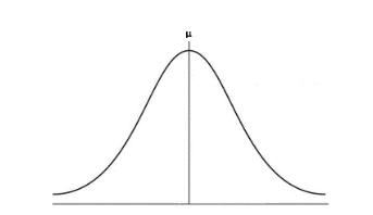
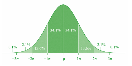
You might have heard of the term ‘bell curve’, a curve that resembles the shape of a bell when plotted on a chart. In statistics, bell curve is frequently used to illustrate normal distribution, which is a type of statistical distribution that is symmetrical about its mean. What does this imply? Well, put it in layman terms, it implies the distribution is shaped identically on both sides of its mean - that is, one half of the distribution will fall to the left of the mean, while the other half will fall to the right. The chart below depicts how a normal distribution looks like – resembling a bell-shaped curve that is spaced evenly on either side of the mean (µ), which is represented by the vertical line.
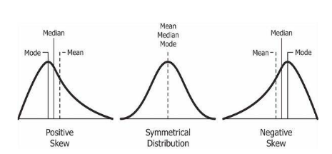
For a distribution that is perfectly symmetrical, the mean will be equal to the median (the midpoint of the data set) and the mode (the observation with the highest frequency). However, if the distribution is asymmetrical, the mean will be either above or below the median and the mode. This can happen when there are outliers (observations with unusually large values) in the data set. If the outliers lie above the mean, the distribution will be positively skewed (right tail is longer than left tail). In this case, the mean will be greater than the median, which in turn will be greater than the mode. On the other hand, if the outliers lie below the mean, the distribution will be negatively skewed (left tail is longer than right tail). In this case, the mean will be less than the median, which in turn will be less than the mode. In short, a positively skewed distribution will have a tail that stretches to the right, while a negatively skewed distribution will have a tail that stretches to the left. The image below shows distributions that exhibit positive skewness, zero skewness, and negative skewness.
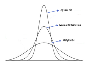
Besides skewness, which measures the extent to which the distribution is asymmetrical, there is another important term called kurtosis. Kurtosis measures the extent to which a distribution is spread out, primarily on the tails. That is, kurtosis tells us whether the data has fatter/longer tails (more observations in the tail) or thinner/shorter tails (less observations in the tail) relative to that of a normal distribution. A normal distribution has a kurtosis of 3. If a distribution has kurtosis greater than 3, it is called a Leptokurtic distribution (longer tails, positive excess kurtosis). Meanwhile, if a distribution has kurtosis less than that of a normal distribution, it is called Platykurtic distribution (thinner tails, negative excess kurtosis). Finally, if a distribution has kurtosis equal to that of a normal distribution, it is called Mesokurtic distribution (zero excess kurtosis). The image below reflects these distributions (leptokurtic, platykurtic, and normal):
A normal distribution possesses the following characteristics:
- Mean = Median = Mode
- Skewness = 0 and Kurtosis = 3
- 50% of the values are less than the mean and 50% are more than the mean
- ~683 out of 1,000 values (i.e., 68.3%) will lie within 1σ from the mean
- ~954 out of 1,000 values (i.e., 95.4%) will lie within 2σ from the mean
- ~997 out of 1,000 values (i.e., 99.7%) will lie within 3σ from the mean
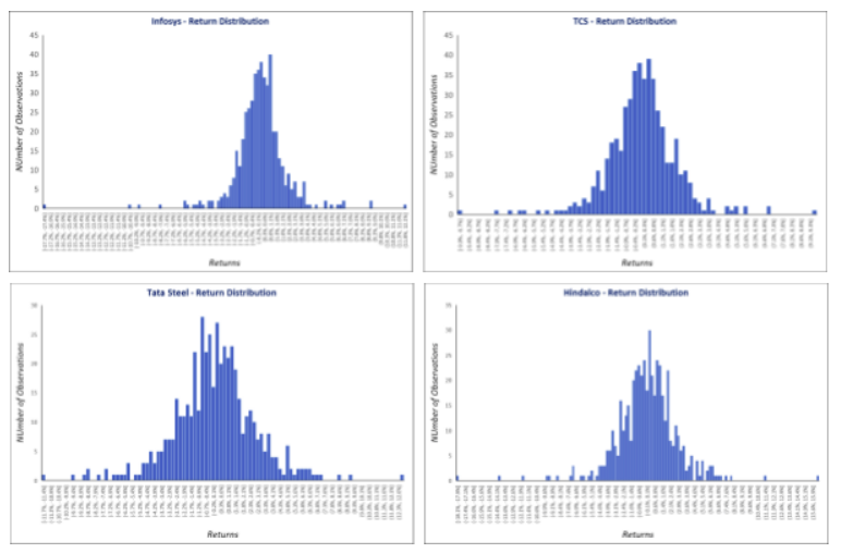
You may wonder why are we discussing concepts such as types of distribution, skewness, kurtosis etc. in this chapter? Well, these concepts are quite important in risk management. Let us start with distribution first. In the financial markets, it is generally assumed that security returns are normally distributed about the mean. To understand this, look at the below histograms:
The above histograms show the daily return distribution of Infosys, TCS, Tata Steel, and Hindalco for the past two years (2019 and 2020). Notice that the bulk of the distribution is concentrated near the center. Also, see how the distribution takes the shape similar to that of a bell curve. Coming back to our earlier discussion, in the financial markets, it is generally assumed that security returns are normally distributed about the mean. This means:
- 68.3% of the returns will lie within ±1σ from the mean (µ - 1σ = 34.1%, µ + 1σ = 34.1%)
- 95.4% of the returns will lie within ±2σ from the mean (µ - 2σ = 47.7%, µ + 2σ = 47.7%)
- 99.7% of the returns will lie within ±3σ from the mean (µ - 3σ = 49.8%, µ + 3σ = 49.8%)
The image above highlights how the data are distributed around the mean (µ) in a normal distribution. See that the bulk of the data are distributed within ±1 standard deviation from the mean. On the other hand, extreme values or outliers that are distributed far from the mean are few in numbers. Positive outliers lie at the right tail (the upper tail), while negative outliers lie at the left tail (the lower tail). As a result, the shape of a normal distribution takes the appearance of a bell curve – being tallest near the mean and then gradually tapering off on either side of the mean. Let us explain this using the hypothetical example of a stock that we presented in the previous chapter, whose mean return (µ) over 10 days was 1.57% and standard deviation (σ) was 4.32%. Based on this information, there is a:
- 68.3% probability that the return on the next day will fall between -2.76% and +5.89%
- 95.4% probability that the return will fall between -7.08% and +10.22%, and
- 99.7% probability that the return will fall between -11.41% and +14.54%
How were the above values arrived at? Well, µ - 1σ = 1.57% - 1*4.32% = -2.76%; µ + 2σ = 1.57% + 2*4.32% = +10.22%, and so on.
Applying μ and σ to identify potential future range:
Continuing with our discussion from the previous section, let us now take a real world example. For our illustration, we have taken the daily log returns of Nifty since the start of 2021 till 23rd March. On this day, the closing price of Nifty was 14814. The table below shows the mean and standard deviation of daily log returns of Nifty for this period.
Based on the above, what do you think will be the range of returns for Nifty over the next one month, which is roughly equivalent to 21 trading sessions? Well, to find that out, we need to convert daily mean and standard deviation to monthly figures. Let us do that right away.
- For calculating monthly μ, we will use the excel formula =(((1+daily μ)^21)-1)*100
- For calculating monthly σ, we will use the excel formula =(daily σ*sqrt(21))
Based on the above formulae, following are the monthly log return statistics for Nifty:
Based on the above table, let us now calculate the possible range of log returns within which Nifty could trade over the next one month.
That said, keep in mind that the above returns are log returns. We need to convert them back to simple returns. To do so, we use the following formula:
We then multiply the above expression by 100 to get simple returns in percentage terms. In the above equation, the expression ‘e’ stands for exponent. It is the base of the natural log and is approximately equal to 2.71828. We can easily solve the above equation in Microsoft Excel using the formula =EXP(log returns)– 1 and then convert it to percent terms to get back the simple returns. Converting the log returns in the above table to simple returns gives us the following statistics:

Now that the returns have been converted back to their initial form, it can be inferred from the above table that over the next one month, there is a:
- 68.3% chance that Nifty returns will range between -3.74% and 8.54% from the closing price of 23rd March (14814)
- 95.4% chance that it will range between -9.34% and 15.25%.
- 99.7% chance that it will range between -14.62% and 22.38%
- 0.3% chance that Nifty returns will be either less than -14.62% or greater than 22.38%
In a similar manner, one could calculate the potential range of returns for Nifty (or for that matter, any other security) for any other period, such as for the next 1 session, next 1 week, next 1 quarter, next 1 year etc. Knowing the probabilistic range of security returns based on mean and standard deviation can help in making assumptions about the expected future returns of a security as well as in gauging potential risks. Based on one’s risk tolerance, it can also help in stock screening and selection.
Skewness and Kurtosis of stock returns:
Earlier in this chapter, we spoke about skewness and kurtosis, which are the third and the fourth central moment, respectively, in statistics (the first is the mean and the second is the variance). When observations in the data set are normally distributed about the mean, one can use standard deviation as an effective measure of risk. That said, keep in mind that standard deviation assumes a distribution that is normal. In the real word however, the distribution of security returns is not always normal. In fact, there is a tendency for security returns to get asymmetric and exhibit skewness and kurtosis. If the returns are asymmetric, then using a model based on normal distribution can lead to an underestimation of risk because these models do not account for extremely large positive or negative returns, such as the ones beyond three standard deviation from the mean. In such a case, skewness and kurtosis would better represent risk.
Let us now look at a real-world example. From the BSE India website, we have downloaded the daily price data of Reliance, Tata Motors, and Wipro from the start of 2021 till date and then performed the following:
- Calculated the log returns of closing prices for each stock
- From the log returns, we have then calculated skewness and kurtosis
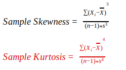
Mathematically, skewness and kurtosis are calculated as follows:
where,
- Xi = ith observation of variable X
- X = the mean
- n = number of observations
- s = sample standard deviation
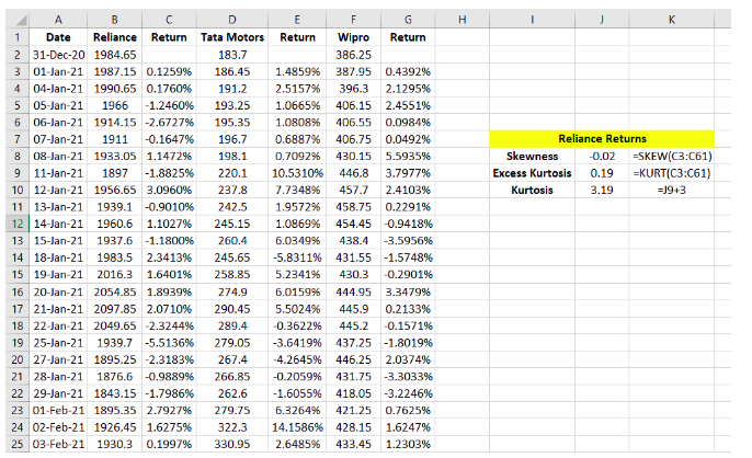
That said, solving for skewness and kurtosis using the above equation is very time consuming and a laborious task. Instead, the simplest way to calculate them is in MS Excel, using the formula =SKEW() for skewness and =KURT() for kurtosis. These calculations can be seen in the below screenshot.
One thing to keep in mind about the =KURT() function in MS Excel is that it calculates excess kurtosis. Recollect that earlier in this chapter we did mention about excess kurtosis. What exactly is this? Well, a distribution is said to exhibit excess kurtosis when its kurtosis is anything but 3, which is the kurtosis of a normal distribution. Mathematically, excess kurtosis is expressed as:
For example, if the kurtosis of a distribution is 7, then excess kurtosis is 7 – 3 = 4; while if the kurtosis if 1, then excess kurtosis is 1 – 3 = -2. As can be seen, excess kurtosis could be positive, zero, or negative.
- If it is positive, the distribution is leptokurtic
- If it is zero, the distribution is mesokurtic
- If it is negative, the distribution is platykurtic
In the above calculation screenshot, notice how the skewness and kurtosis have been calculated based on the daily log returns of Reliance (see the formula used for calculating skewness and excess kurtosis in cell K8 and K9, respectively). The table below highlights the key statistics for each stock:
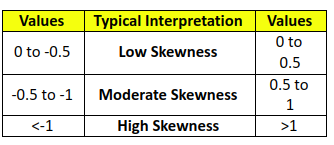
In the above table, notice that Tata Motors had the highest standard deviation as well as the highest excess kurtosis. This means that since the start 2021 till the time of writing, compared to the other two stocks, Tata Motors not only had higher dispersion around the mean return but also had longer tails. Furthermore, a moderate level of positive skewness suggests that the returns of Tata Motors are right-skewed.
For return distributions that are leptokurtic (long-tailed distribution), there will occasionally be instances of abnormally extreme returns on either side of the mean, that is returns that are outside three standard deviations from the mean. A leptokurtic distribution accompanied by negative skewness (left-tailed distribution) implies at a greater risk, because of the higher odds of negative outliers. On the other hand, a leptokurtic distribution accompanied by positive skewness (right-tailed distribution) implies at a higher odds of positive outliers. This sort of distribution is something that would suit an aggressive investor. Meanwhile, for return distributions that are platykurtic (short-tailed distribution), the outliers would be smaller than those found even in normal distribution. When accompanied by low to moderately positive skewness, such distributions would imply at stable returns and low risk. This sort of distribution is something that would suit a conservative investor.
In the next chapter, we will continue our discussion of statistical measures of risk by talking about covariance and correlation.
Next Chapter
Comments & Discussions in
FYERS Community
