Over the last four chapters, we studied some important statistical tools that help in measuring risk and return. To reiterate, following are the statistical metrics we have covered so far in this module:
- Arithmetic and geometric mean
- Variance and standard deviation
- Distribution of security returns
- Skewness and kurtosis
- Covariance and correlation coefficient
- Beta
That said, each of the concepts that we have discussed so far were based on measuring the risk and return of an individual security. In this chapter, we will talk about measuring the risk and return of a portfolio of securities.
Expected Return on a security
Before proceeding towards discussing portfolio risk and return, let us first understand how to calculate the expected return on a security.
Approach 1: Calculating the expected return based on historical returns:
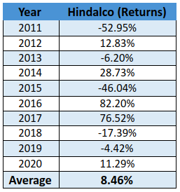
In an earlier chapter, we discussed about calculating the mean return of a security based on the security’s historical returns data. Well, this is one way in which the expected return on a security can be calculated – using historical data to measure how much you can expect to earn, on average, in the future. Let us understand this using the annualized simple returns of Hindalco over the past ten years:
Based on the historical yearly returns data, the average annual return of Hindalco for the past ten years turned out to be 8.46%. So, going forward, in a typical year, based on the historical data, it can be inferred that the expected return on Hindalco would be around 8.46%.
Approach 2: Calculating the expected return using CAPM:
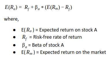
Another way of calculating expected return on a stock is using the Capital Asset Pricing Model (CAPM) approach. This model helps an investor calculate the expected return on a security for a given level of market risk, measured using Beta. Under the CAPM approach, the expected return on a security can be calculated using the following formula:
The expression E(Rm)-Rf in the above equation is also known as the equity risk premium. Multiplying the equity risk premium by beta compensates the investor for taking the appropriate level of systematic risk beyond the risk-free rate of return. The higher the beta, the higher would be the expected return, and vice versa. This is because the higher the beta, the higher would be the systematic risk. Hence, to compensate for higher systematic risk, an investor would demand a higher return as well.
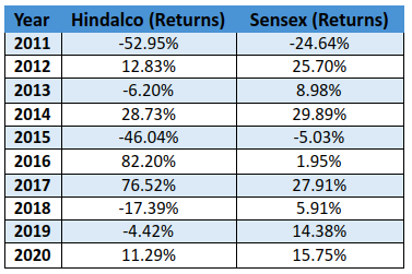
Let us understand this using the annualized simple returns data of Hindalco (the dependent variable) and Sensex (the independent variable) over the past ten years:
Based on the above statistics of the past 10 years, the following has been calculated:
- Beta of Hindalco = 1.63
- Sensex annual average return = 10.08%
What about the risk-free rate? Well, in our case, because we are using a 10-year data, we could take yield on the 10-year G-sec as the risk-free rate. Why G-secs? Well, because these instruments are issued by the Indian government and hence are considered very safe. As at the end of 2020, the yield on India’s 10-year G-Sec was 5.9%. Now that we have all the three variables, let us calculate the expected return of Hindalco using the above CAPM equation.
The additional return over 5.9% is the excess return that an investor would demand to compensate for the additional risk he or she would be taking for investing money in a stock (Hindalco in our case). See that the higher the beta, the higher does this additional return turn out to be, and vice versa.
Besides statistical metrics, fundamental and/or technical parameters can also be used to calculate the expected return on a security.
Expected Return of a portfolio:
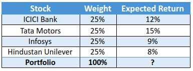
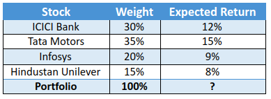
Now that we understand how to calculate expected return of a stock, let us move ahead and talk about the expected return of a portfolio. Let us assume an investor has a four stock portfolio. Let us also assume that capital deployed is ₹1 lac, split evenly among the four stocks. Following are the details of the portfolio:
For ease of illustration and to just focus on the concept in hand, the expected stock returns that we have mentioned in the table above are random numbers. When investing however, these would be based on fundamental, technical, and/or statistical parameters. Based on the individual stock weights and individual expected returns, the portfolio expected return can be calculated as:
Above, notice that the weight of each stock has been multiplied with the respective expected return. Each of these values are then summed to arrive at the portfolio return. Keep in mind that the weights of stocks in the portfolio must exactly add up to 100%.
On the other hand, what if the weights were not equal. What if the weights were as follows:
Using the same logic as above, the portfolio return can be calculated as:
Portfolio Variance and Standard Deviation
Now, let us talk about how to calculate portfolio variance and standard deviation. After all, return is only one component. The other critical and arguably more important component is risk. How do you calculate the portfolio risk?
Now, let us talk about how to calculate portfolio variance and standard deviation. After all, return is only one component. The other critical and arguably more important component is risk. How do you calculate the portfolio risk?
Well, one of the most common ways of measuring the portfolio risk is by calculating the portfolio variance and standard deviation. However, the calculation of portfolio variance is not as straight forward as calculating portfolio return. We cannot simply multiply the weight of each stock by the respective variance and then sum all these values together. Instead, variance of a two-stock portfolio is calculated as:
Taking the square root of the above equation gives us the standard deviation as follows:
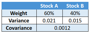
Let us assume the following details for two stocks, A and B:
Using the above statistics, let us now calculate the variance and standard deviation of the portfolio:

So, the standard deviation of the above 2-stock portfolio is 10.26% Now, what if you wanted to calculate the variance of a three-stock portfolio? Well, for a three-stock portfolio, the variance is calculated as:
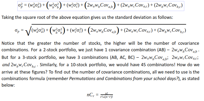
In the above equation, C stands for Combination and the symbol ‘!’ denotes factorial. Because we have 10 stocks and we want to find out all the possible covariance combinations (each of which is calculated between 2 stocks), n=10 and r=2. Substituting these values in the above equation, we get,

Now how do we solve for 10!? Well,
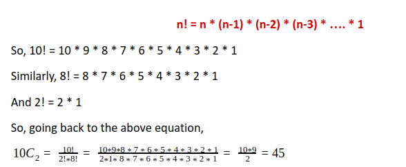
Using the above formula, now try to calculate the number of combinations that would be needed to calculate the variance for a 20-stock portfolio (Answer is 190). Imagine performing so many calculations manually. That would be quite a daunting task, isn’t it?
As you can see, calculating the variance of a two-stock portfolio is not quite hard but is a little time consuming. However, as the number of stocks increase, calculating portfolio variance manually can become extremely complex and time consuming. Hence, it is better to calculate portfolio variance in Microsoft Excel rather than doing it manually. In the next chapter, we shall talk about how to calculate portfolio variance and other important portfolio calculations in Microsoft Excel. So, stay tuned!
Portfolio Beta
Let us now talk about portfolio beta and how to calculate it. In the previous chapter, we spoke about the beta of a stock. Just to reiterate, beta measures the sensitivity of stock returns to that of the market. Portfolio beta, meanwhile, measures the overall sensitivity of a portfolio of stock returns to that of the market. It is calculated as the weighted average of the beta of individual stocks, as shown below:
Let us understand this using a portfolio of four stocks. The weights of these stocks and their individual beta (versus Sensex) based on the returns for the period between 1st January to 20th April 2021 have been mentioned in the table below:
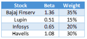
Based on the above statistics, the portfolio beta turns out to be:

What can we interpret from the above value? Well, the portfolio beta of 1.01 tells us that the portfolio is as volatile as the market (recollect, the beta of the market is 1). In other words, if the market rises by 10%, the portfolio is also likely to gain by around 10%; while if the market falls 3%, the portfolio is also likely to fall by around 3%.
Again, keep in mind that the weights of stocks must add up to 100%.
Next Chapter
Comments & Discussions in
FYERS Community
