
By now, we know how to calculate individual stock and portfolio risk and return, both manually and in Microsoft Excel. In this chapter, we will discuss portfolio optimization strategies and talk about the ways in which one can fine tune a portfolio with the objective of minimizing risk for a given level of return.
Minimum Variance Portfolio and the Efficient Frontier:
Over the past few chapters, we spoke about how to calculate portfolio expected return and variance. When it comes to portfolio, one of the key factors that affect risk and return are the security weights. For instance, if stock A has a standard deviation of 30% and stock B has a standard deviation of 45%, then assigning a greater weight to stock B than to stock A would cause the portfolio volatility to be higher than if higher weights were assigned to Stock A. So, selecting the right weights based on one’s risk tolerance and reward expectations is critical when it comes to portfolio management. Up until this chapter, whenever we chose stock weights, we did so randomly. In this chapter however, we will look at techniques that can be used to optimize a portfolio by fine tuning weights.
Let us assume that an investor has chosen to deploy capital in HDFC Bank and Tata Steel. Now that the stock selection is done, the next step is capital allocation between the two stocks. Based on the daily price data, below are the statistics for each stock over the last 1 year (29-April-20 to 26-April-21):


Above, we have calculated the portfolio expected return and standard deviation for one possible combination: 40% HDFC Bank and 60% Tata Steel. Is this combination of stock weight the most ideal? Well, there is no way to say that at hindsight. Instead, to find that out, stock weight combinations must be jotted down, and the portfolio expected return and standard deviation must be calculated for each of these combinations. Keep in mind, the total weight must add up to 100%.
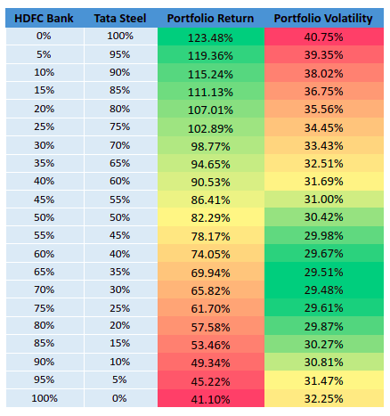
From the above combinations, notice that the lowest portfolio volatility, or risk, is 29.48%. At this level, the expected portfolio return is 65.82%. This risk and return occur at the 70% HDFC Bank and 30% Tata Steel combination. We can also plot the same on a scatter graph. To do so on Microsoft Excel, click on the Insert tab and then within the Charts ribbon, select Scatter chart. This has been shown in the image below:

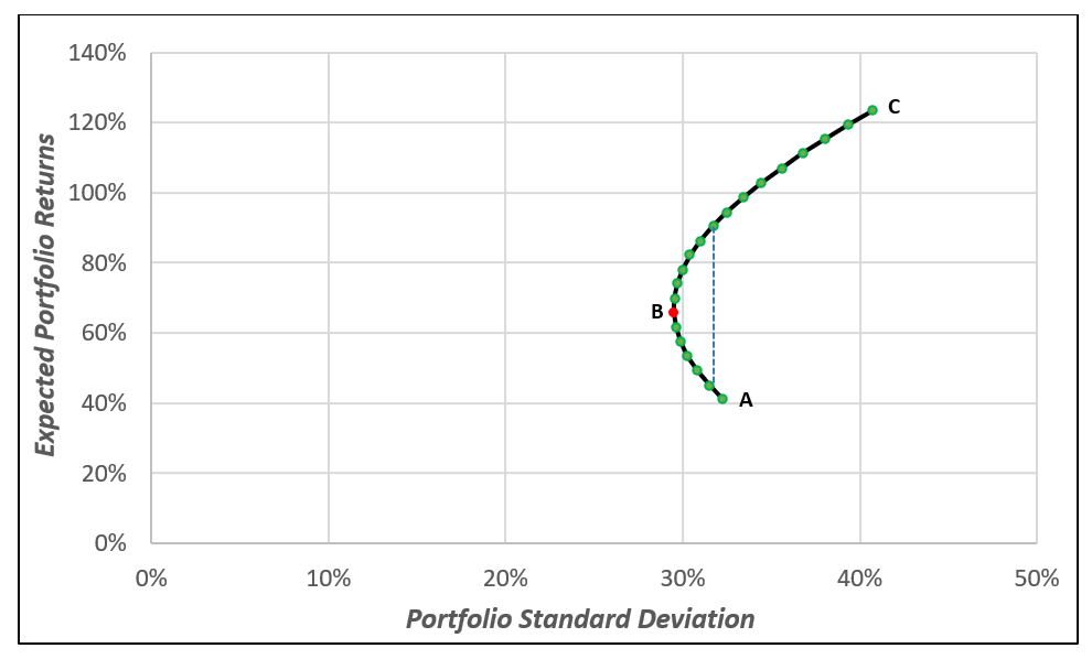
Above, the X-axis represents the standard deviation of the portfolio, while the Y-axis represents the portfolio expected returns. The curve that you see in the graph above is commonly referred to as the Portfolio Possibilities Curve. Let us now briefly explain this graph.
- Point A represents the point with the lowest possible return. It occurs when 100% of capital is deployed in HDFC Bank. In this case, because the entire capital is going into HDFC bank, the expected return and standard deviation of the portfolio would be equal to that of HDFC Bank. See that no diversification would be achieved in this case.
- As the proportion of capital allocation increases in Tata Steel and decreases in HDFC Bank, see that the curve will start shifting to the left and move higher until it reaches point B. At point B (70% HDFC Bank and 30% Tata Steel), the portfolio risk would be the lowest (29.48%). Above point B, see that the curve will start shifting to the right and continue moving higher until it reaches point C.
- Point C represents the point with the highest possible return but see that this also comes with the highest possible risk. It occurs when 100% of capital is deployed in Tata Steel. As a result, the expected return and volatility of the portfolio would be equal to that of Tata Steel. Again, see that no diversification would be achieved in this case.
In the above table and graph, we have performed just a few portfolio combinations, in multiples of 5%. In reality, however, there would be infinite such combinations between 0-100%. Manually doing this, however, would not be possible. Later, we will talk about how to do this in Microsoft Excel.
The point that lies at the extreme left on the portfolio possibilities curve is the point with the lowest portfolio standard deviation. This point is known as the Global Minimum Variance Portfolio. No portfolio combination would produce a portfolio risk lower than the one at this point. In the above chart, however, keep in mind that point B is not exactly the global minimum variance portfolio, because we have considered only a handful of portfolio combinations rather than all combinations.
All points that lie on the curve but above the global minimum variance portfolio are known as the Efficient Frontier. The efficient frontier comprises of all the efficient portfolios that provide the highest return at each level of risk. Meanwhile, portfolio combinations that lie on the curve but below the global minimum variance portfolio comprises of inefficient portfolios. What does all of this mean? Well, keep in mind that for a given level of risk, any rational investor or trader would want to earn the highest possible return. Alternatively, for a given level of return, they would want the lowest possible risk. With this in mind, go back to the chart above and notice the two points that the horizontal dashed blue line connects. Here, we have two combinations. Both the combinations offer a similar risk (31.47% vs. 31.69%). However, observe that the combination that lies above the global minimum variance portfolio has an expected return of 90.53% while the one that lies below the global minimum variance portfolio has an expected return of 45.22%. Let us summarize this up in the table below:

From the above table, it is logical to assume that one would prefer the second combination as it offers a much higher expected return for essentially the same level of risk as the first combination. It is for this reason that points lying above the global minimum variance portfolio comprise of efficient portfolios, while those lying below comprise of inefficient portfolios.
On the efficient frontier, there is no specific preferred portfolio combination. Instead, this depends on the individual risk-taking ability and reward expectations of an investor. An aggressive investor, who believes in taking greater risks, might prefer a portfolio combination that is higher and towards the right of the efficient frontier. On the other hand, a conservative and a risk-averse investor might prefer a portfolio combination that lies closer to the global minimum variance portfolio.
Portfolio Optimization on Microsoft Excel:
Now that we understand global minimum variance portfolio, how to approximately find it, and the efficient frontier, let us focus on how to find the most optimal portfolio combination with the objective of minimizing portfolio standard deviation. In other words, let us find the global minimum variance portfolio. This can be done on Microsoft Excel using the Solver function. To open Solver, click on the Data tab and then click on Solver, as shown in the image below:

If you are unable to find the Solver function in the Data tab, perform the same steps that we explained for adding the Data Analysis function in chapter 10. Let us continue with our example of HDFC Bank and Tata Steel. Earlier, we found out that an allocation of 70% in HDFC Bank and 30% in Tata Steel produces the lowest portfolio standard deviation. However, this was based on just a select few portfolio combinations rather than all. To find out the portfolio allocation that produces the lowest standard deviation of all the possible portfolios, we need to perform the following:
- First, calculate the return and standard deviation for both the stocks. Also, create a covariance matrix (using the Data Analysis toolpak and then transpose to fill blank cells).
- Next, create a table for weights. For now, leave the individual weights unfilled and create a row for calculating the total weight. Then, sum the weights of the stocks. As the individual weights have not been filled, the total weight should show up as 0 after inputting the formula.
- Lastly, input the formulas to calculate the expected return and portfolio standard deviation. As the individual weights have been left blank, you will get the ‘#VALUE!’ error. At this point, do not worry about this error.
All this, including the formulas used, has been shown in the image below (carefully go through the formulas used to calculate total weight, portfolio expected return, and portfolio standard deviation). Also note that after populating the covariance matrix using the Data Analysis toolpak, another covariance matrix has been created to annualize all the covariances. This has been done by multiplying each covariance by 250:
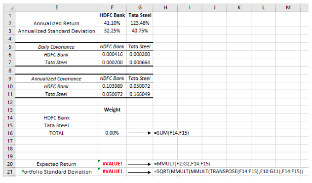
The reason why we have left the individual weights blank is because we would want Excel to solve the most ideal portfolio combination for us such that the portfolio standard deviation is minimized. Now, the next step is to click on the Solver button. Once the Solver dialog box opens, perform the following:
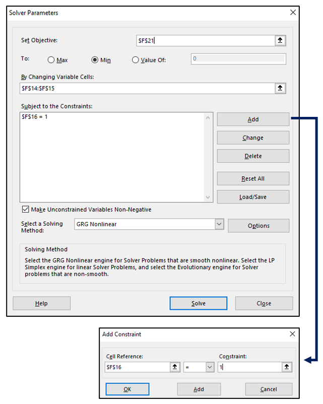
- In the first dialog box (Set Objective), click on the cell where we have inputted the portfolio standard deviation formula. In case of the image above, see that this falls in cell F21.
- In the next dialog box (To), because we are interested in finding the lowest possible standard deviation, click on Min
- In the next dialog box (By Changing Variable Cells), select the cells that contain the weights of the individual stocks. In case of the image above, this happens to be cells F14:F15.
- In the next dialog box (Subject to the Constraints), click on Add. In the new dialog box that opens, do the following:
- In Cell Reference, select the cell that contains the total of the weight. In case of the image above, this happens to be the cell F16
- In the next drop down menu, choose the sign =
- In Constraint, type in 1 (what this means is the total of the weight is set to 100%). Finally, select OK. You will notice that the constraint has been added
- Now that we have inputted all the necessary variables, click on Solve. The Solver Results dialog box will open. Click on OK.
For ease of understanding, all the aforementioned steps can be seen in the images below:
Let us now display the results below:
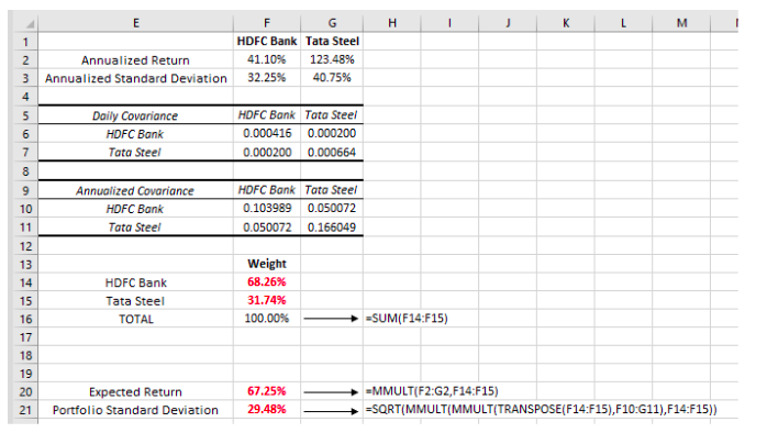
As can be seen in the image above, the lowest possible portfolio standard deviation that can be attained by deploying capital in HDFC Bank and Tata Steel is 29.48%. This is achieved when 68.26% of the capital is allocated to HDFC Bank and 31.74% is allocated to Tata Steel. Also see that the expected portfolio return corresponding to this standard deviation is 67.25%.
Let us now try out another example. Let us say that Mr. A has chosen four stocks in which to deploy his money – SBI, Lupin, Wipro, and Graphite. Based on the daily price data, below are the statistics for each of these stocks over the last 1-year (29-April-20 to 26-April-21):
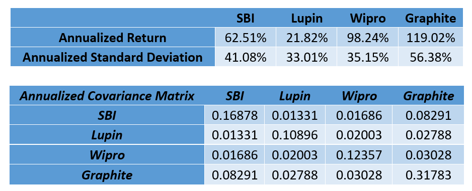
Now, Mr. A wants to find out how to allocate capital among these stocks, such that the portfolio standard deviation reduces to as great an extent as possible for a given expected return. Let us do that now using the Solver function. The results have been displayed below:
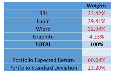
As can be seen in the table above, the lowest attainable portfolio standard deviation is 23.20%. The expected return of the portfolio corresponding to this volatility is 60.64%. Let us now focus on the stock weights. See that Lupin has the highest weight of 39.41% while Graphite has the lowest weight of 4.23%. But what if Mr. A wants to allocate a minimum and a maximum threshold to the weight of each stock? For instance, what if Mr. A wants to allocate at least 10% and at most 35% in each of the stock? Well, this can also be performed using the Solver function, by adding constraints.
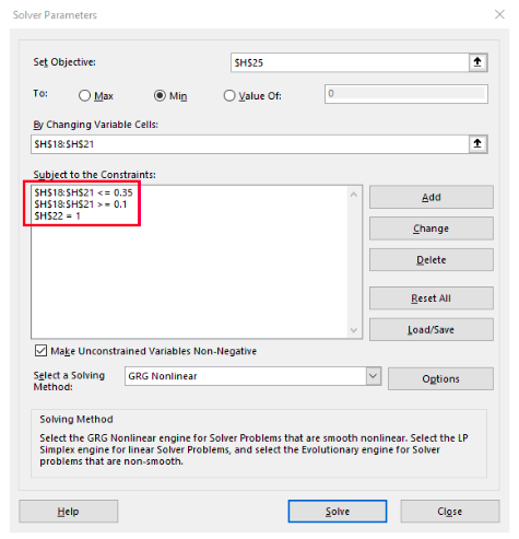
Notice the highlighted constraints in the image above. See that the maximum weight per stock is 35% and the minimum weight is 10%. Now, let us look at the results below:
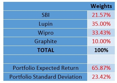
As can be seen, the weight allocation has changed. Because of this, there is a slight change in risk and expected return as well. See that the portfolio standard deviation has increased slightly to 23.42%, while the expected return has gone up to 65.87%. This way, depending on your objective, you can fine-tune the portfolio by adding multiple constraints in the solver function. Furthermore, similar to the manner in which we found out what portfolio combination would minimize the portfolio volatility, we can also find out what portfolio combination would maximize the expected return.
In the next chapter, we will continue our discussion on portfolio and talk about the various statistical ratios that can be used to measure risk and return.
Next Chapter
Comments & Discussions in
FYERS Community