
In this chapter, we will talk about some key statistical ratios that can be used to measure and compare the risk and return characteristics of a portfolio (and individual securities too).
Coefficient of Variation
So far, we have not yet talked about Coefficient of Variation. Let us start this chapter by discussing about it. Let us assume an investor wants to choose between two stocks: HDFC Bank and Tata Steel. Based on the daily log returns, following are some statistics for each of these stocks over the last one year (29-April-20 to 26-April-21):

From the above table, it can be seen that the annualized return on HDFC Bank is quite less than that on Tata Steel. At the same time, the risk (as measured by standard deviation) is only marginally lower. While there are various parameters that affect the selection criteria of stocks, for now, let us just focus on individual stock risk and return and ignore the rest. Based on the above statistics, which of the two stocks are better picks? Well, one way to determine this is to calculate Coefficient of Variation (or CV), which measures the risk per unit of return. CV is calculated as follows:

As can be seen, the numerator comprises of risk while the denominator comprises of returns. The lower the ratio, the lower would be the dispersion around the mean, which would imply a lower risk (or volatility) per unit of return. Hence, the lower the ratio, the superior is the risk to return trade-off. Let us calculate CV for the above two stocks:

So, based on the past year’s data and just the individual stock risk and return criteria, Tata Steel would be a better choice between the two as it offers a superior risk-return trade-off.
Coefficient of Variation is a simple statistic that can help in quickly measuring risk to reward, and in the process help in choosing between two or more securities. However, keep in mind that while standard deviation can never be negative, the mean return can be negative. And when the mean return is negative, this statistical tool is not of much use. This is because when the mean return is negative, so is the CV, which does not make much sense.
Sharpe Ratio
Let us assume there are two portfolios: A and B. Let us say portfolio A and B have earned an average annual return of 10% and 12%, respectively, over the last 3 years. If you had to put money in one of the two portfolios, which would you prefer? Well, at hindsight, portfolio B looks the better choice, because of the higher returns it offers. However, remember, return is only one side of the equation. The other side is risk. Without knowing what the corresponding risk is, a decision cannot be taken. What if the higher return generated by portfolio B has coincided with it experiencing a much higher volatility than portfolio A during the same period? Well, in that case, portfolio B might not be a better choice, especially for those who are risk averse. Hence, it is not just about the returns, but also about the risk that is assumed to earn returns. One way is to combine both risk and return to calculate the risk-adjusted return. This is what each of Sharpe and Treynor ratio does. Let us start our discussion with the Sharpe ratio.
Sharpe ratio is one of the most widely used ratios to measure the risk-adjusted returns. It measures the excess return of a portfolio (or a market proxy or an individual security, etc.) relative to its risk. It is expressed as:
.png)
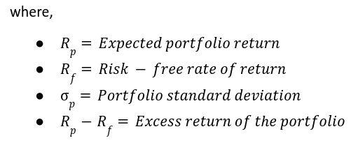
As can be seen from the above equation, Sharpe ratio measures the excess return of a portfolio per unit of total risk (standard deviation). Naturally, the higher the ratio, the better. Typically, a value below 1 implies that the excess return generated by the portfolio over the risk-free return does not compensate for the risk being taken. Hence, it is considered poor. Meanwhile, a value above 1 implies that the excess return generated by the portfolio compensates for the risk being taken. The higher the value above 1, the more attractive is the risk-adjusted return. Because Sharpe ratio takes into consideration the total risk, which includes both systematic and unsystematic risk, it can be measured for even those portfolios that are not well-diversified.
Sharpe ratio does not offer as much an insight when used in isolation as it does when used to compare the risk-adjusted returns of different portfolios. For instance, if the Sharpe ratio of portfolio A is 1.05 and that of portfolio B is 1.50, it tells that portfolio B has a better return-to-risk trade-off than portfolio A. Sharpe ratio is also useful when an investor wants to find out the sort of impact there would be on the risk-adjusted portfolio return when introducing a new stock into the portfolio. If doing so causes the Sharpe ratio to increase, it tells the investor that introducing that stock would improve the risk-adjusted return of the portfolio. However, if doing so causes the Sharpe ratio to decline, it tells the investor that he or she could be better off by not introducing that stock into the portfolio.
Treynor Ratio
Another ratio that is widely used to measure the risk-adjusted return is the Treynor ratio. This ratio is quite similar to the Sharpe ratio. The only difference is that instead of using the standard deviation of portfolio returns, it uses the beta of the portfolio. It is expressed as:

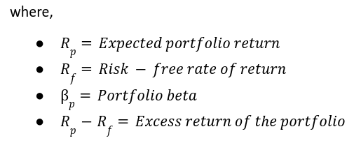
Compare the above formula with that of Sharpe ratio. You will notice that the only difference lies in the denominator. While Sharpe ratio takes into consideration the overall risk, Treynor ratio takes into consideration only the systematic risk. Hence, before using the ratio, it must be ensured that the portfolio is well-diversified, as Treynor ratio does not account for the unsystematic risk. Just like in case of Sharpe ratio, the higher the Treynor ratio, the better. Treynor ratio can offer valuable insights when comparing portfolios or when finding out the sort of impact there would be on the risk-adjusted portfolio return when introducing a new stock into the portfolio.
Illustrating Sharpe and Treynor ratio using a real-world example
Now that we understand Sharpe and Treynor ratio, let us look at a real-world example. Let us assume that there are three portfolios: A, B, and C. Portfolio A comprises of HDFC Bank, Tata Steel, and Lupin; portfolio B comprises of SBI, Wipro, and Tata Motors; and portfolio C comprises of Bajaj Finserv, Balkrishna Industries, and Graphite. For simplicity’s sake, let us also assume that each portfolio is equi-weighted (i.e., 1/3rd weight to each stock). Based on the daily log returns, following are some statistics for each of these stocks and portfolio over the last one year (29-April-20 to 26-April-21):
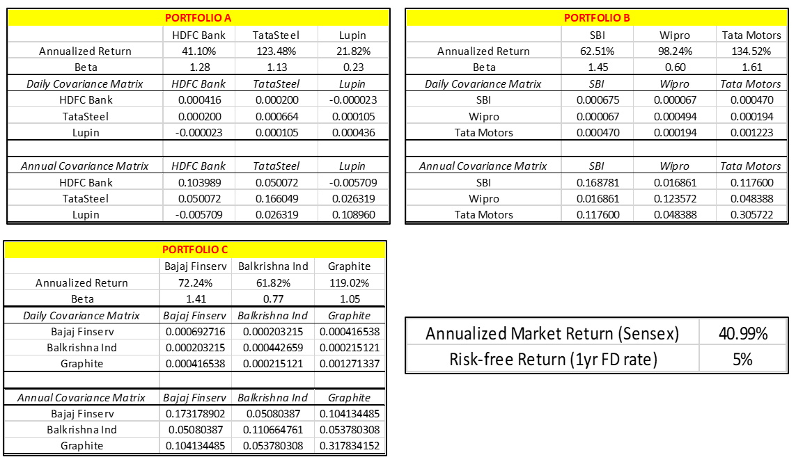
Based on the above individual values, the following portfolio values have been calculated:
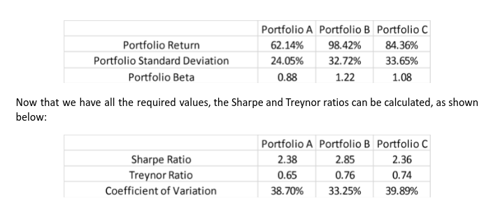
What can we infer from the above? Well, see that portfolio B not only offers the highest return, but it also offers the highest risk-adjusted returns. See that of the three portfolios, portfolio B has the highest Sharpe ratio as well as Treynor ratio. Hence, from a risk-adjusted standpoint, if a choice has to be made over which one of the three portfolios to deploy capital, then it must be portfolio B. Also notice that portfolio B has the lowest coefficient of variation.
Portfolio Optimization using Sharpe and Treynor ratio:
By now, we know that the Sharpe and Treynor ratio can be used to measure the risk-adjusted returns of a portfolio. We also know that the higher the ratio, the better, because it implies at a higher risk-adjusted return. This knowledge can be used to optimize a portfolio and allocate stocks weights that would cause the Sharpe ratio to maximise. From our discussions in the previous chapter, recollect that we can optimise a portfolio using the Solver function in Microsoft Excel. Let us do that again now.
In the example that we spoke about earlier in this chapter, we assigned an equal weight of 33.33% to each stock in a portfolio. The screenshot below highlights that example:
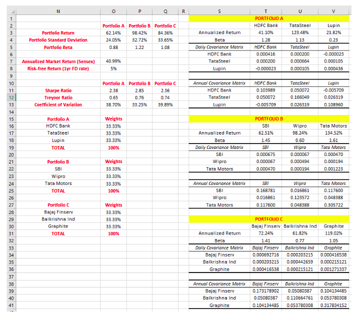
Now, let us see how to allocate weights that would cause the Sharpe ratio to maximise. Let us focus on portfolio A. As can be seen in the image above, a weig ht of 33.33% has been assigned to each stock that is a part of portfolio A (HDFC bank, Tata Steel, and Lupin). Let us now go to the Solver function and perform the following steps:
- In Set Objective, select the cell that contains the Sharpe ratio of Portfolio A, as our objective is to maximise this cell. In case of the image above, that cell happens to be O11.
- In By Changing Variable Cells, select the cells that contain the individual stock weights of portfolio A. In case of the image above, that cell happens to be cells from O16:O18.
- Click on Add button in Subject to the Constraints. Within Cell Reference, select the cell that contains the total of the weight of portfolio A. In case of the image above, that cell happens to be O19. In the next drop down menu, select =. Finally, in Constraint, type in 1 (or 100%). Then click on OK.
- Finally, click on Solve button. Once the Solver Results window pops up, click on OK. The results of the optimisation have been displayed below:
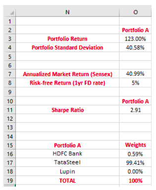
See that the maximum attainable Sharpe ratio in case of Portfolio A is 2.91. This is achieved when 99.4% of the capital is allocated to Tata Steel and the rest is allocated to HDFC bank, with no allocation going into Lupin. Notice that along with the Sharpe ratio, the portfolio return has also gone up, but so has the standard deviation. It can be seen that although the Sharpe ratio is maximized, the portfolio is not at all diversified as virtually the entire capital has been allocated to a single stock. Hence, further optimization is needed to achieve diversification and reduce the unsystematic risk of the portfolio. This can be done by assigning minimum and maximum weight to each stock in the portfolio. To do that, all you need to do is add two more conditions in the Solver function, one for assigning a minimum weight per stock and the other for assigning a maximum weight. Let us allocate a minimum weight of 20% and a maximum weight of 40% to each stock. The new results have been displayed below:
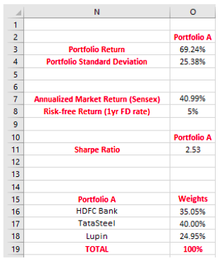
By assigning a minimum and a maximum weight of 20% and 40%, respectively, to each stock in portfolio A, see that the Sharpe ratio now stands at 2.53. While this ratio is lower than the one we saw in the previous scenario wherein over 99% of the weight was assigned to Tata Steel (2.91), see that the ratio is higher than the scenario wherein equal weights were assigned to each stock (2.38). Notice that to achieve this Sharpe ratio, 40% of the capital was allocated to Tata Steel, 35% to HDFC Bank, and the remaining 25% to Lupin. Furthermore, compared to the original portfolio wherein equal weights were assigned to each stock, see that the portfolio return has gone up (69.24% vs. 62.14%), while the portfolio standard deviation has increased only marginally (25.38% vs. 24.05%). For ease of comparison, all the three tables have been displayed below.

Similarly, you could perform the calculations for portfolios B and C with the objective of maximizing the Sharpe ratio. A certain weight threshold could also be assigned to ensure that an extremely high weight is not assigned to any one particular stock and that diversification is achieved. Meanwhile, using the same logic, one could also optimise the portfolio with the objective of maximizing the Treynor ratio. Let us do this for portfolio B (SBI, Wipro, and Tata Motors) using the following three scenarios:
- Each stock is assigned an equal weight of 33.33%
- The Treynor ratio is maximized without any minimum and maximum stock weight threshold
- The Treynor ratio is maximized under the condition that each stock has a weight of minimum 20% and maximum 40%
As you are already aware of how to use the Solver function, let us directly display the results below:

The image on the left displays the results when all the three stocks are assigned an equal-weight. Meanwhile, the maximum Treynor ratio that can be attained is 1.56, shown in the middle image. See that this happens when the entire capital is allocated to Wipro. While this provides the highest return per unit of systematic risk, it is not an ideal combination because doing so provides no portfolio diversification whatsoever and exposes one to unsystematic risk. Furthermore, the significant decline in portfolio beta would cause the portfolio to underperform the markets, especially during times of a bull market. Finally, the image on the right displays the results when each stock is assigned a minimum and a maximum weight of 20% and 40%, respectively, in portfolio B. Compared to the scenario wherein equal weights are assigned to each of the three stocks, see that assigning a 20% weight to SBI and a 40% weight to each of Wipro and Tata Motors increases the Treynor ratio to 0.86. Furthermore, also see that the portfolio return has increased to 105.61%.
Well, that was all that we wanted to talk about in this chapter.
Phew! Over the last eight chapters, we discussed some heavy yet critical statistical and Microsoft Excel-related concepts that one needs to be aware of. We started by discussing statistical metrics at the individual-stock level and then proceeded to discuss them in detail at the portfolio level. Well, these were all the key statistical concepts that we wanted to speak about in this module. Going forward, from the next chapter, we will turn our attention to trading and discuss key risk-management concepts pertaining to trading, including stop losses, targets, risk-to-reward ratio, and position sizing.
Next Chapter
Comments & Discussions in
FYERS Community