In the previous chapter, we discussed how to calculate the expected return on a portfolio. We also spoke about how to calculate portfolio variance and standard deviation as well as the beta of a portfolio. However, we did so manually, which can become quite cumbersome and time consuming if there are more than 2-3 stocks in a portfolio. In this chapter, we will continue our focus on what we spoke about in the last few chapters. However, we will talk about how to do so in Microsoft Excel, so as to reduce the quantum of manual work and save on time.
Calculating Correlation Matrix in Microsoft Excel:
In chapter 7, we spoke about correlation. Back then, we spoke of how to calculate correlation between just two stocks. But what if there are multiple stocks, which would make it necessary to calculate several correlation pairs? This is indeed a situation in case of a portfolio, which comprises of 3 or more stocks. While the number of stocks in a portfolio can vary from one investor or trader to another, typically, an ideal portfolio comprises between 8 to 20 stocks. Let us assume an investor wants to build a diversified portfolio comprising of 5 stocks – A, B, C, D, and E. Because the investor wants to diversify, he or she would be interested in knowing the correlations between all the pairs of stocks. How many pairs of correlation can we calculate for a 5-stock portfolio? Well, this can be solved using the combinatorics formula that we discussed in the last chapter. The answer is 10 – AB, AC, AD, AE, BC, BD, BE, CD, CE, and DE. As there are 10 pairs of correlation, analyzing them would be much simpler if done using a correlation matrix. Let us understand how to create a correlation matrix in Excel using the 1-year daily log returns data of the following ten stocks: HDFC bank, SBI, Tata Steel, Lupin, Wipro, Tata Motors, Bajaj Finserv, Dabur, Balkrishna Industries, and Graphite.
Step-1:
Download the 1-year daily price data of each of the above stocks. You could do so from either the NSE or the BSE website. Ensure that the data is sorted date-wise.
Step-2:
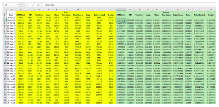
Once the data has been downloaded, calculate the daily log returns for each stock. A portion of the price and returns data has been shown in the image below:
Step-3:
Once the returns for each stock have been populated, the next step is to create a correlation matrix. To do so, click on the Data tab. Then, within the data tab, if you look to the far right, there will be an option called ‘Data Analysis’ within the Analyze ribbon. This has been shown in the image below and highlighted in red:
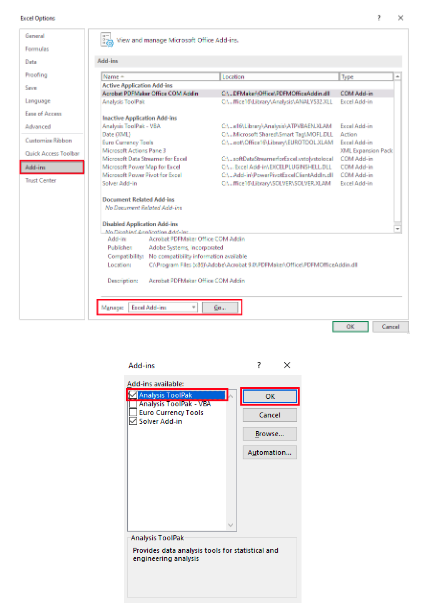
If the Data Analysis option is not visible, do not worry. You can enable it by clicking on File Options. Within Options, click the Add-ins tab. To the bottom of the Add-ins dialog box, there will be a drop-down menu that reads Manage. Within this drop-down menu, choose Excel Add-ins and click on Go. This will open the Add-ins dialog box. Tick the Analysis ToolPak option and then click on OK.
Then go back to the Data tab and select Data Analysis. There are various statistical calculations that can be performed quite quickly and efficiently using the Data Analysis ToolPak. Because we are interested in calculating correlations, click on the Correlation button within the Data Analysis dialog box and select OK. This will open the Correlation dialog box.
Step-4:
Within the Correlation dialog box, you need to do three things as follows:
- First, select the ‘Input Range’. To do so, select all the cells that contain the returns data, including the row that contains stock names.
- Next, tick the ‘Labels in First Row’ option.
- Finally, tick the ‘Output Range’ option and then select any blank cell where you would want the output to be displayed.
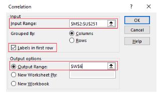
Once each of these three things have been inputted, select OK. The correlation matrix would now be populated. Below are the results of the correlation:

You could also perform conditional formatting and color the cells to easily identify which stocks share strong correlation and which share weak correlation. In the above table, the color of the cells varies from dark green (which represents stocks sharing the highest correlation) to dark red (which represents stocks sharing the lowest correlation).
Within the context of portfolio diversification, a correlation matrix is an important table. It lets one understand the extent of correlation between all the possible pairs of stocks that are a part of the portfolio. A portfolio that has a strong positive correlation (such as above 0.5, on average) is indicative of poor diversification and therefore is inherently riskier. On the other hand, a portfolio that has a strong negative correlation (such as below -0.5, on average) is over diversified and therefore would compromise on the return potential. Hence, it is important to strike a balance between a portfolio that is poorly diversified and one that is over diversified. This also applies to the number of stocks in a portfolio (very few stocks would indicate at poor diversification, while too many stocks could indicate at over diversification). A well-diversified portfolio is one that has low to moderate correlation (such as between 0 and 0.5, on average). Such a degree of diversification would help in reducing portfolio risks, particularly the ones that are unsystematic in nature.
Calculating Covariance Matrix in Microsoft Excel:
In a similar manner in which we calculated the correlation matrix, we can calculate the covariance matrix as well. To do so, again go to the Data tab and within that select Data Analysis. Once the Data Analysis dialog box pops up, select Covariance. Then, within the covariance dialog box, perform the following:
- Select the Input Range
- Tick the ‘Labels in First Row’ option
- Select the Output Range
Finally, click on OK.
Doing so would populate the covariance matrix. Below are the results of the covariance matrix for the same set of data that we presented when explaining the correlation matrix.
That said, keep in mind that the covariance matrix calculated using the Data Analysis ToolPak represents the population covariance rather than sample covariance. There will be minor differences in values between the two. Meanwhile, the blue cells in the table above reflect covariance of a stock with itself, which, as we know by now, is nothing but the variance of the stock. So, as we can see, all the blue cells in the table above are variances, while the rest are all covariances. It is for this reason that a covariance matrix is referred to as a variance-covariance matrix as well.
Calculating Portfolio Variance in Microsoft Excel:
Finally, let us now turn our attention towards portfolio variance. As we saw in the last chapter, when there are more than 2-3 stocks in a portfolio, which is typically the case, calculating the portfolio variance becomes quite complex and time consuming. Hence, the most optimal way to solve for portfolio variance is in Microsoft Excel. To calculate portfolio variance in Excel, all that we need are individual stock weights and all the covariance pairs. Let us understand this using the same example of the 10-stock portfolio discussed earlier in this chapter. We have already calculated the covariance matrix in the previous section. Let us again paste that matrix here.
When plotting the covariance matrix using the Data Analysis ToolPak, all the duplicate entries are ignored, as can be seen in the table above where all the cells that are above the blue coloured cells are blank. The reason why these are blank is because they are duplicates of entries that have already been made in the filled cells that are below the blue coloured cells. For instance, notice that cell B3 displays the covariance of HDFC bank and SBI. However, see that the corresponding duplicate entry has been left blank in cell C2, which represents the covariance of SBI and HDFC bank. Recollect from our earlier chapter: covariance of stock A and B is the same as covariance of stock B and A.
Having said that, to calculate portfolio variance, the first thing that we need to do is to populate the entire table above by filling all the blank cells as well. To do so, all that we need to do is transpose the entries from each column to the corresponding row.
For example, to transpose the vertical entries from cells B3 to B11 horizontally across the cells C2 to K2, we use the function =TRANSPOSE(B3:B11) in the cell C2. Doing so would paste all the vertical entries from B3 to B11 horizontally across C2 to K2. To understand this better, look at the image below. See that by inputting the transpose function in cell C2 (look at the formula bar), the cells from C2 to K2 get populated using the corresponding entries from cells B3 to B11.

Similarly, to transpose the vertical entries from cells C4 to C11 horizontally across the cells D3 to K3, we use the function =TRANSPOSE(C4:C11) in the cell D3, as shown below:
We do this in the same manner until all the corresponding empty cells are filled. The final populated covariance matrix has been posted below:
Now that the covariance matrix has been populated by filling all the blank cells, the next step is write down the stock weights for each of the 10 stocks. Below mentioned are the weights that we have assigned for each stock:
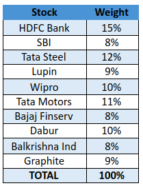
Ensure that the total weight adds up to 100%. Now that we have both the individual stock weights and the covariance matrix, the final step is to calculate the portfolio variance. In the image below, see how we have calculated the portfolio variance and annualized standard deviation.
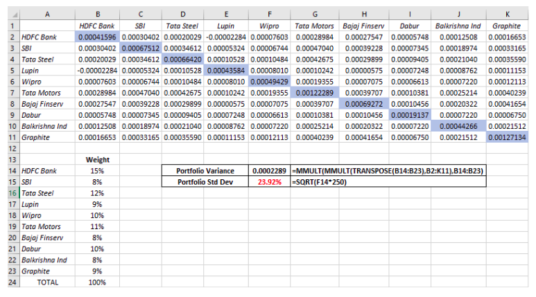
As can be seen in cells F14 and F15, the portfolio variance and annualized standard deviation are 0.0002289 and 23.92%, respectively. Kindly notice the Excel formulas used above to calculate the variance. At first sight, the formula might look quite intimidating. But do not worry, we shall simplify this in the next section.
Understanding Excel’s MMULT function to solve for Portfolio Variance:
In the previous chapter, we spoke about a formula that can be used for calculating portfolio variance. However, using that formula is feasible only if the portfolio comprises of 2 or 3 stocks. If a portfolio comprises more than 3 stocks, solving using that formula becomes complex and time consuming. Hence, an ideal way to solve for portfolio variance is in Excel, using the function MMULT. This function is used to multiply two matrices. That said, before speaking about the MMULT function, one needs to understand the basics of matrix. To learn about matrix, we suggest you visit the following links:
Coming back, from a matrix perspective, portfolio variance is expressed as:
In the above equation, W refers to the column vector of stock weights. It is the third matrix that consists of a single column. Meanwhile, Wt refers to the transpose of stock weights (row vector). It is the first matrix that consists of a single row. Finally, covariance matrix refers to all the possible pairs of covariances. Keep in mind that the order mentioned in the above equation is important – first matrix is the row vector of stock weights, second matrix is the covariance matrix, and third matrix is the column vector of stock weights.


Above, the 1st matrix is multiplied by the second matrix. This resulting product is then multiplied by the 3rd matrix.
When multiplying two matrices, the number of columns in matrix 1 must equal the number of rows in matrix 2. It is for this reason that the first matrix of stock weights is transposed, so that the number of columns in the weight matrix matches with the number of rows in the covariance matrix. Let us understand this using a simple, hypothetical example of two stocks. Below, the table on the left represents the weight and that on the right represents the covariance matrix.

When expressed in the form of a matrix, the above tables would look like the ones below:

Above, in case of the matrix on the left, there are two rows and one column. As such, this is a 2 by 1 (or 2x1) matrix. Meanwhile, in case of the matrix on the right, there are two rows and two columns. As such, this is a 2 by 2 (or 2x2) matrix. Keep in mind, a matrix is expressed in the form M by N, where M refers to the number of rows and N refers to the number of columns. So:
- Matrix 1 = 2x1 matrix
- Matric 2 = 2x2 matrix
Recollect what we said earlier. When multiplying two matrices, the number of columns in matrix 1 must equal the number of rows in matrix 2. Above, however, matrix 1 consists of 1 column while matrix 2 consists of 2 rows. Because of this mismatch, we need to transpose matrix 1, so that it then becomes a 1x2 matrix and can then be multiplied with matrix 2.
Rather than doing manually (which can get quite laborious and time consuming), this calculation can be quickly done in Excel using the =MMULT(A,B) function, where A represents array 1 (the 1st matrix) and B represents array 2 (the 2nd matrix). Let us do that below:
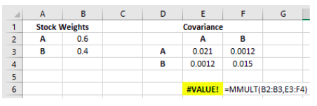
Before we explain the above image, here is an important thing to keep in mind. If you are using the latest version of Microsoft Office 365, you can directly hit enter after inputting all the required arrays in the MMULT function to generate the output. However, if you are using any other version of Microsoft Office, you may need to press Shift + Control + Enter to generate the output.
Now, in the above image, notice the highlighted cell E6 and the formula that was used to calculate this, in cell F6. As you can see, we got an error (#VALUE!). The reason why we got an error is because the number of columns in the weight matrix (1) did not match with the number of rows in the covariance matrix (2). Hence, we need to transpose the weights, so that the matrix changes from a 2x1 to a 1x2 matrix. So, let us work again.

The result of the product of the two matrices has been calculated in cell E6 and the formula that was used to calculate this has been written in cell G6. Notice that multiplying a [1x2] matrix with a [2*2] matrix results in a [1x2] matrix, as can be seen in the highlighted cells E6 and F6.
Now, this resulting product must be multiplied by the third matrix (which is the column vector of stock weights) to get the value of the portfolio variance. Let us do that below:
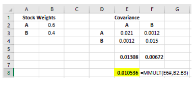
In the above image, notice the highlighted cell E8 and the formula that was used to calculate this in cell F8. See that the resulting product (E6#), which is a [1x2] matrix (E6:E7), is multiplied by the column vector of stock weights, which is a [2x1] matrix. Notice that multiplying a [1x2] matrix with a [2*1] matrix results in a [1x1] matrix, as can be seen in the highlighted cell E8. This value, 0.010536, is nothing but the portfolio variance.
Instead of using the function MMULT twice, we can further shorten our work by nesting an MMULT within another MMULT. To understand how to do this, look at the image below:

In the above image, notice the highlighted cell E6 and the formula that was used to calculate this in cell F6. Notice how MMULT has been nested inside another MMULT, to directly generate the portfolio variance.
As we know from our discussions from the previous chapters, variance is not much useful by itself. What is instead more valuable is standard deviation. We know that standard deviation is nothing but the square root of variance. So, let us now calculate portfolio standard deviation from the portfolio variance arrived at in the above image.

Now that you understand how to calculate portfolio variance using the MMULT function, it is time to go back to our earlier example of the 10-stock portfolio and understand how the MMULT function was used. The image has been repasted below:
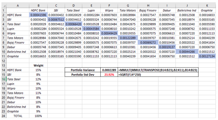
The variance that we get, 0.0002289, is based on daily stock returns. Taking the square root of this gives us a standard deviation of 0.01512962. Keep in mind that this is the daily standard deviation. To annualize it, we multiply this value by the square root of 250, which gives us 0.239220301, or 23.92%.
While all this may sound intimidating, it is not. In fact, once you understand how to use the MMULT function, you would be in a position to calculate portfolio variance within minutes, no matter how many stocks the portfolio comprises of. All that you need to do is populate the covariance matrix using Excel’s Data Analysis toolpak and have the stock weights ready, before using the MMULT function.
Next Chapter
Comments & Discussions in
FYERS Community
