By now, we know the basics of risk as well as the various risks that investors and traders are exposed to. In this chapter as well as in the next few, our objective is to explain various statistical ways of measuring and quantifying risk and return. In this chapter, we shall talk about:
- Arithmetic Mean and Geometric Mean
- Variance and Standard Deviation
- Simple returns versus Log-based returns
Arithmetic and Geometric Mean
Mean, or average, is the most widely used measure of identifying the central point of a data set. In finance, it is primarily used for calculating the average return for a given number of observations in the data set. The most widely used form of mean, known as arithmetic mean, is calculated as follows:
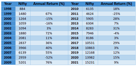
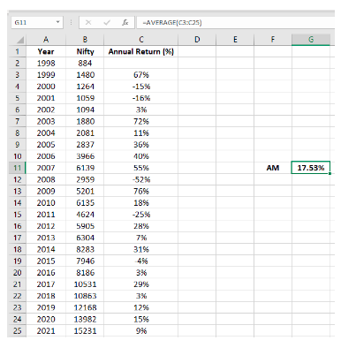
The above table shows the annual returns of Nifty for each of the past 23 years. To find out the average annual return of Nifty since 1999, all you need to do is add up each of the annual returns and then divide by 23. Accordingly, you would get the average annual return of Nifty since 1999 as 17.53%. You do not need to do this manually. Instead, you can solve this using the =AVERAGE() function on Microsoft Excel, as shown in the screenshot below:
Sometimes, you may be more inclined towards calculating compounded returns, especially in cases where the returns are reinvested rather than withdrawn. In such cases, geometric mean is used rather than arithmetic mean. Geometric mean can be calculated using the following formula:
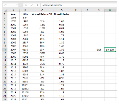
Manually calculating the geometric mean can be quite a dauting and time-consuming task. Hence, the best way to solve for geometric mean is using the = GEOMEAN() function on Microsoft Excel. When doing so, one should not forget to add 1 to each period return and finally subtract 1 from the output, as shown in the formula above. To understand this better, look at the below screenshot.
Above, the growth factor for each period is nothing but 1 + annual return. Finally, observe the formula bar to understand how the geometric mean is calculated in cell H11. See that 1 has been subtracted from the output. So, the geometric mean or the compounded annual returns of Nifty for the past 23 years is 13.17%.
See above that the geometric mean is less than the arithmetic mean. In fact, whenever there is dispersion in data (returns in our case), the geometric mean will always be less than the arithmetic mean. Furthermore, the larger the dispersion, the larger will be the difference between arithmetic and geometric mean (former being higher than the latter). For instance, in the above case of Nifty, if you observe each of the annual returns, you will see there is quite a bit of difference over the years. As such, the arithmetic return is notably higher than the geometric return. The only instance when the two will be equal is when there is no dispersion in the data set.
Which is better: Arithmetic or Geometric Mean?
Well, that depends. If each data within a data set is not dependent on one another, arithmetic mean should be preferred. For instance, let us say that a student has scored 80% in English, 95% in Mathematics, and 90% in Science. In this case, a simple average would suffice as the individual scores are independent. Similarly, if an investor has earned a 15% return on stock A, 18% on Stock B, and 7% on stock C, arithmetic mean would suffice to calculate the average return on the three stocks (we will talk about portfolio returns in a later chapter). Arithmetic mean can also be used when dispersion between observations is relatively negligible. However, when observations within a data set are dependent on one another and the deviation between observations is anything but negligible, geometric mean should be preferred. In the world of finance, when calculating return on an investment, geometric mean is mostly preferred over arithmetic mean. This is because the returns generated between periods are correlated. Let me explain this using a simple example.
A security generated a return of +20% in the 1st year and -20% in the 2nd year. In this case, the annualized arithmetic mean return would be 0%, which would suggest that the security yielded no return over a two-year period. But is this true? Let us say that ₹100 was initially invested. This ₹100 would have amounted to ₹120 at the end of year 1 and ₹96 at the end of the year 2. So, at the end of the 2nd year, the investor would have suffered a loss of 4% on his/her invested capital of ₹100. Meanwhile, the annualized geometric mean return for the same investment would be -2.02%. See that the geometric mean reflects this loss and thereby offers a more accurate picture than the arithmetic mean. Hence, in cases where returns are reinvested, geometric mean should be preferred over arithmetic mean, as the latter tends to overestimate returns when there is dispersion in the data.
Importance of Mean in Statistics:
In statistics, mean is one of the most used metrics to calculate the center of the data set. Not only is the mean widely used by itself, but it also forms a critical part of several other statistical metrics and calculations. In finance, the mean is widely used to calculate historical returns of a security, which then forms the basis for calculating expected returns on a security as well as a portfolio. The mean is also used to compare returns between securities and assets, so as to make trading and investment choices. Further, the mean forms a critical component of measuring the distribution of security returns as well as in calculating a range of risk measurement tools. Hence, because of its widespread application in finance and statistics, it is important to have a thorough understanding of the mean as it pretty much forms the base of statistical analysis.
Before proceeding, let us consider a hypothetical situation. Let us say that over the last six months, stock A, B, and C have generated an average monthly return of 1.5%, 2%, and 1%, respectively. Based on this data, if one is looking for a trading opportunity, which of the three stocks should be selected? Well, at hindsight, it might be easy to say stock B, for the simple reason that it has generated the highest return of the three stocks. Well, this is not necessarily true. Always keep in mind that returns represent only one half of the trade. The other half is represented by risk. Without knowing what the risk is, a conclusion should not be reached. Hence, before choosing one of the three stocks based on historical returns, one must see how the returns have fluctuated (risk) in the past. The most common way to do this is to measure standard deviation, which is the topic of discussion in the next section.
Variance and Standard Deviation:
In the previous section, we talked about mean return, which is also the realized historical return of a security. We spoke about how arithmetic and geometric mean help us in calculating average returns, be it on an annualized basis or on any other basis. However, keep in mind that mean return does not show the complete picture. It tells nothing about the degree to which the returns vary over time. To understand this, let us go back to the previous example. If you look at the table, you will see that Nifty has generated a mean annual return of 17.53% over the past 23 years. However, if you closely observe, you will notice that the returns each year have fluctuated substantially from as low as -52% to as high as +76%. Because the returns are volatile, there is an element of uncertainty and risk involved.
The variability in returns, which is nothing but risk, can be measured by a few statistical tools, one of which is variance and standard deviation. Variance is used to measure the average dispersion in the data set around a central value - the mean. In other words, variance shows how far the observations are scattered around the mean. The farther the observations are from the mean, the larger will be the variance (and therefore volatility), and vice versa. Statistically, variance is the average of the squared distance between each observation and the mean, whereas standard deviation is the square root of variance. This may sound a little intimidating, but it is not. Let us simplify this by showing the steps that are involved in the calculation of variance and standard deviation of the returns of a security:
- Step 1: Calculate the stock return for each data point
- Step 2: Calculate the mean of the values arrived in step 1
- Step 3: Calculate the difference between each observation arrived in step 1 and the mean arrived in step 2
- Step 4: Square each of the differences arrived in the step 3
- Step 5: Calculate the total of the squared differences arrived in step 4
- Step 6: Divide the total arrived in step 5 by (n – 1)
The figure that is arrived in step 6 is the sample variance. To calculate the population variance, you will have to divide the figure arrived in step 5 by just ‘n’ and not ‘n-1’. That said, in most of the cases, because a sample is used to represent the population, sample variance is calculated rather than population variance. Going one step further will yield standard deviation, as shown below:
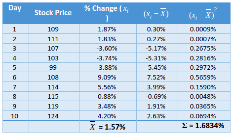
Let us now understand the calculation of variance and standard deviation using a hypothetical example. For our purpose, we will calculate variance and standard deviation of the returns of stock XYZ over the past 10 sessions.
- Step 1: Calculate the percent change of each data. In the example above, we will calculate the percent price change of each session using the formula: {(Current day price ÷ Previous day price) – 1} *100. The results have been shown in Column 3 of the above table.
- Step 2: Calculate the average of all the observations arrived at in step 1. In our case, the average return turns out to be 1.57%.
- Step 3: Calculate the difference between each observation (xi) arrived in step 1 and the mean (X) arrived in step 2. The results (xi-X) have been shown in Column 4 of the above table.
- Step 4: Square each of the differences arrived in step 3. The results have been shown in Column 5 of the above table.
- Step 5: Calculate the sum of all squared observations that were arrived in step 4. In our case, this value turns out to be 1.6834%.
- Step 6: Divide the value arrived in step 5 by 9 (number of observations – 1) to calculate the sample variance. In our case, the sample variance turns out to be 0.1870%.
- Step 7: Finally, calculate the standard deviation by taking the square root of variance. In our case, standard deviation turns out to be 4.3249%.
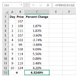
So, this is how variance and standard deviation are calculated. The steps involved are quite simple, but the calculation is cumbersome and time consuming. The good news is you do not need to perform so many steps. Instead, Microsoft Excel can do all the hard work for you. All you need is do is:
- Download data of historical prices for the period for which you are looking to calculate variance and standard deviation (You could download from NSE, BSE, or Yahoo Finance).
- Calculate the percent change of each period.
- Finally, calculate the standard deviation using the =STDEV function (If you are also interested in calculating variance, use the =VAR() function).
In the image above, see the formula bar to understand how standard deviation has been calculated in cell C13. So, the mean return of this security over the past 10 days is 1.57% while the standard deviation is 4.32%. What this tells us is that over the past 10 days, the average deviation, or the average distance, of returns from the mean is 4.32%. In isolation, standard deviation may not provide much information about volatility. However, when compared with that of other securities, standard deviation will shed a lot of information about the past volatility.
So far, we have based our calculation of variance and standard deviation on returns (i.e., percent change in price). However, variance and standard deviation can be calculated on absolute price also. In the case of the above example, if the calculations are done based on the price itself (and not returns), the mean would be ₹110.9, variance would be 54.99, and standard deviation would be ₹7.42.
Annualizing Standard Deviation:
Above, we calculated the standard deviation of returns based on the daily closing price. So, the figure that we arrived at was the standard deviation of daily returns (based on the past 10 sessions). In other words, we arrived at the 1-day standard deviation for the past 10 sessions. However, standard deviation is generally expressed in annualized terms. So, what if we wanted to convert the standard deviation based on daily returns to annualized standard deviation? Could we do it? Well, the answer is yes. To convert standard deviation based on daily returns to annualised standard deviation, we can use the following formula:
In the above equation, 250 represents the approximate number of trading sessions in a year. In a similar way, if returns are based on weekly prices, the number inside the square root in the above equation would be 52; if they are based on monthly prices, the number inside the square root would be 12; if they are based on quarterly prices, the number inside the square root would be 4; and if they are based on semi-annual prices, the number inside the square root would be 2.
So, coming back to our previous example of stock XYZ, the standard deviation was 4.3249%. This is the standard deviation based on daily returns. Using the above formula, the annualized standard deviation turns out to be 68.38% (=4.3249*SQRT(250)).
On the other hand, what if you instead had annualized standard deviation and wanted to convert it to, say, daily standard deviation? In that case, you would manipulate the above formula as follows:
In the above case, to convert annualized volatility of 68.3822% to daily volatility, you would perform the following calculation in Excel: =68.3822÷SQRT(250)
Simple returns versus lognormal returns:
In the hypothetical example of stock XYZ that we spoke about earlier in this chapter, we calculated standard deviation of stock returns based on simple returns. That is, we calculated the return for each period using the formula mentioned below and then took the average of those returns:
However, simple return has an inherent problem as shown in the illustration below:
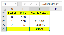
In the above image, see that the security price has risen 20% at the end of the 1st period and then declined 20% at the end of the 2nd period. Calculating the average of these returns generates a mean return of 0%, which kind of suggests that the investor has neither made money nor lost money. However, if you closely notice, the investor has realized a loss of 4%. See that if ₹100 was invested at the start of the period, it would be worth ₹96 at the end of the 2nd period. This is the issue posed by simple return because it does not take into consideration the effects of continuous compounding. As such, it tends to overestimate the returns. Logarithmic return, on the other hand, takes continuous compounding into its calculation. Look at the image below to understand this:
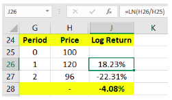
See cell J26 and then focus on the formula bar to understand how the log return is calculated for each period. It is calculated on Microsoft Excel using the following function:
In the above expression, LN stands for the function, natural log. The log returns of each period can be summed to figure out the overall log return, something which cannot be done in case of simple returns. For instance, the overall log return for the above example can be solved as =LN(96/100), which turns out to be -4.08%. This gives the same result as adding the log returns for period 1 (18.23%) and 2 (-22.31%). However, with simple return, see above that adding +20% and -20% results in 0, while calculating the overall simple return over 2 periods results in -4% (((96÷100)-1)*100). Also, log values are more suitable when measuring changes in a variable that follows normal distribution. As it is generally assumed that stock returns tend to follow normal distribution, log values are hence more appropriate. It is because of these reasons that standard deviation of stock returns must be based on log returns rather than simple returns. We will talk about normal distribution in the next chapter. Let us now go back to our earlier example of stock XYZ and calculate standard deviation based on log returns.
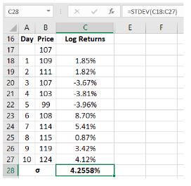
In the above example, notice that the log returns are calculated for each period rather than simple returns, using the Excel function =LN(). The standard deviation is then calculated in cell C28, as can be seen in the formula bar above. Using log returns, the standard deviation turned out to be 4.2558%, as compared to 4.3249% that was the case when simple returns were used. Do keep in mind that this is the daily standard deviation. To calculate the annualized standard deviation, you need to multiply the daily standard deviation with the square root of 250. In this case, the annualized standard deviation turns out to be 67.2895%.
Let us conclude this discussion by highlighting the results in the table below:
Real world application of Standard Deviation on stocks:
Now that we have understood how to calculate standard deviation, let us take a real-world example. Let us take four stocks - two from the IT sector (Infosys and TCS) and two from the metal sector (Tata Steel and Hindalco). Let us calculate the volatility of each of these stocks for 2019 and 2020. To do so, perform the following:
- Download the daily historical data of each stock from 31st Dec 2018 till 31st Dec 2020. You could download the same from the BSE website, the NSE website, or from Yahoo Finance (Click here to download historical stock data from BSE, click here to download historical index data from BSE, and click here to download historical index data from NSE)
- Once you have downloaded the data, calculate the log daily return of each stock for both 2019 and 2020 (ensure that the data is in ascending order, date-wise)
- Calculate the mean and standard deviation based on the log daily return values
- Also calculate the annualised mean and standard deviation from the respective daily mean and standard deviation values
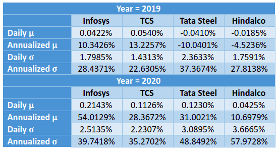
The statistics are as mentioned in each of the tables below, with the table on the top representing the statistics for 2019 while that at the bottom representing the statistics for 2020.
You may wonder, how did we calculate the annualized mean in each of the above tables. Well, because we already had the log-based return for the entire year (both 2019 and 2020), the annualized mean was calculated as the summation of all the log returns for each of the four securities and for each period. Remember from our earlier discussion, log returns can be summed.
If you go through the above tables, you will see that the two IT stocks exhibited less deviation from the mean return than did the two metal stocks in each of the past two years, more so in 2020. In other words, IT stocks were less volatile than metal stocks during the stated period.
Knowing historical volatility can help a trader or an investor in choosing the right securities for trading or investing depending on his/her risk profile and objectives. Typically, a conservative trader or investor would be more inclined towards choosing securities that exhibit less volatility, so as to reduce exposure to risks. On the other hand, an aggressive trader or investor could be more comfortable choosing stocks that exhibit high volatility, as high volatility also means the possibility of earning higher-than-average returns.
As a side note, before we conclude this chapter, let us quickly understand how to convert daily return to annualized return. What if the average daily return of a security, say for the month of March, is 0.05% and you want to annualize it? How would you do that?
Well, you could do so using the below formula:
So, inputting 0.05% in the above equation, we get annualized return as 13.31%. Similarly, to calculate the quarterly return based out of the daily mean return, replace 250 in the above formula with 63 (because there are approximately 63 trading days in a quarter); to calculate the monthly return based out of the daily mean return, replace 250 with 21 (because there are approximately 21 trading days in a month), and so on.
Importance of Standard Deviation in Finance:
In finance, standard deviation is one of the most widely used metric to measure risk. It enables traders and investors to understand how volatile a security has been over the period under consideration. A high standard deviation tells that there has been a larger deviation in the returns of a security from its mean return, while a low standard deviation tells that there has been less deviation in the returns of a security from its mean return.
Keep in mind that a high standard deviation is not necessarily bad, just as a low standard deviation is not necessarily good. Instead, it all depends on the risk appetite and reward expectations of traders and investors. A trader or an investor who has a higher risk appetite and reward expectations would be happy to deploy funds in securities that exhibit high standard deviation. On the other hand, a trader or an investor who has a lower risk appetite would prefer deploying funds in securities that exhibit low standard deviation. Always keep in mind, higher the standard deviation, higher would be the risk but so would be the reward potential, and vice versa.
Furthermore, standard deviation and volatility can also be used to determine the extent of stop losses for a trade. We will talk more about this in a later chapter.
Things to keep in mind about Standard Deviation (σ):
Standard deviation is a tool that is very widely used not only by itself but also as a part of other metrics used to measure individual and portfolio risks. We will continue talking about standard deviation over the next few chapters.
Let us wrap up this chapter by highlighting the key properties of standard deviation:
- σ is the most used metric to measure risk in an investment (or a trade)
- σ can be either positive or zero, but can never be negative
- A σ of zero means there is no dispersion in the data set
- A σ greater than zero means there is dispersion in the data set
- The higher the σ, the higher the volatility and therefore risk, and vice versa
- σ is expressed in the same unit as the mean. As a result, it is a more widely used metric than variance
- Because σ utilizes mean in its calculation, it is heavily influenced by outliers
- In finance, σ can be calculated based not only on price returns but on absolute price as well
- σ of stock returns must ideally be calculated on lognormal returns rather than simple returns
- σ can be compared across securities, such as stocks, sectors, indices etc.
- Usually, blue chip stocks tend to have low σ as compared to midcap or smallcap stocks
Next Chapter
Comments & Discussions in
FYERS Community



.png)


