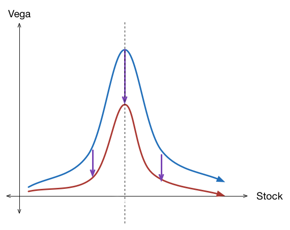
Over the next two chapters, we will come across one of the most referred to word in the options parlance - Implied Volatility (IV). We shall talk about what it is and how it is related to the Option Greek, Vega. In our previous two chapters, we briefly talked about how volatility impacts Delta and Gamma. Now, in this chapter and in the next, we shall focus on Vega and see how it impacts the price of an option. Besides, we shall also discuss about the two most used measures of volatility - Historical and Implied. Needless to say, one must have a strong understanding of volatility, given that it strong influences option price and the types of option strategies that are deployed by a trader. So, without any further ado, let us get started.
Volatility and Standard Deviation
Before dwelling into Vega, let us first understand what volatility is. Put it in simple words, volatility is the rate at which the price of an asset fluctuates over time. An important thing to keep in mind regarding volatility is that it tells nothing about the direction in which the price of the asset is moving. Instead, it just tells the magnitude of fluctuation in the price of the asset. The higher the volatility, the higher is the magnitude of the fluctuation in price, and vice versa. A very commonly used measure of volatility in the financial world is standard deviation.Let us now talk more about this.
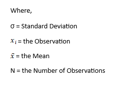
Standard Deviation, denoted by the Greek letter σ, measures the amount of dispersion around the mean, wheremean is the average of the observations within the data set over the past ‘n’ periods. Standard deviation is calculated using the formula as below:
.png)
Let us now see how standard deviationis calculated. For our example, we shall use the 30-trading daysdaily price and returns data of the Nifty 50 index (price data taken from Yahoo Finance):
| Date | Nifty | Daily % Change (  |
 |
 |
| 21-11-2019 | 11968 | -0.256% | -0.320% | 0.0010% |
| 22-11-2019 | 11914 | -0.451% | -0.516% | 0.0027% |
| 25-11-2019 | 12073 | 1.337% | 1.273% | 0.0162% |
| 26-11-2019 | 12037 | -0.299% | -0.363% | 0.0013% |
| 27-11-2019 | 12100 | 0.523% | 0.459% | 0.0021% |
| 28-11-2019 | 12151 | 0.417% | 0.353% | 0.0012% |
| 29-11-2019 | 12056 | -0.783% | -0.847% | 0.0072% |
| 02-12-2019 | 12048 | -0.065% | -0.129% | 0.0002% |
| 03-12-2019 | 11994 | -0.448% | -0.513% | 0.0026% |
| 04-12-2019 | 12043 | 0.409% | 0.344% | 0.0012% |
| 05-12-2019 | 12018 | -0.206% | -0.270% | 0.0007% |
| 06-12-2019 | 11921 | -0.806% | -0.871% | 0.0076% |
| 09-12-2019 | 11937 | 0.134% | 0.070% | 0.0000% |
| 10-12-2019 | 11856 | -0.676% | -0.740% | 0.0055% |
| 11-12-2019 | 11910 | 0.450% | 0.386% | 0.0015% |
| 12-12-2019 | 11971 | 0.518% | 0.453% | 0.0021% |
| 13-12-2019 | 12086 | 0.960% | 0.895% | 0.0080% |
| 16-12-2019 | 12053 | -0.271% | -0.335% | 0.0011% |
| 17-12-2019 | 12165 | 0.921% | 0.857% | 0.0073% |
| 18-12-2019 | 12221 | 0.466% | 0.401% | 0.0016% |
| 19-12-2019 | 12259 | 0.311% | 0.247% | 0.0006% |
| 20-12-2019 | 12271 | 0.099% | 0.034% | 0.0000% |
| 23-12-2019 | 12262 | -0.074% | -0.138% | 0.0002% |
| 24-12-2019 | 12214 | -0.393% | -0.457% | 0.0021% |
| 26-12-2019 | 12126 | -0.720% | -0.785% | 0.0062% |
| 27-12-2019 | 12245 | 0.983% | 0.919% | 0.0084% |
| 30-12-2019 | 12255 | 0.082% | 0.018% | 0.0000% |
| 31-12-2019 | 12168 | -0.713% | -0.778% | 0.0060% |
| 02-01-2020 | 12282 | 0.935% | 0.870% | 0.0076% |
| 03-01-2020 | 12226 | -0.452% | -0.517% | 0.0027% |
 |
0.064% | Ʃ  |
0.1050% | |
Now that we know what the numerator of the expression is, the standard deviation can be calculated using the above mentioned formula as:
So, the standard deviation of Nifty daily returns for the past 30-trading sessions is 0.60%. What this means is that the daily returns of Nifty have fluctuated ~0.60% from their mean return of 0.06% over the past 1-month. In the financial world, standard deviation is mostly annualized and expressed in percentage terms. Doing so standardizes the number, thereby enabling one to compare the standard deviation across securities. To annualize the standard deviation of daily returns, multiply the standard deviation by the square root of the number of trading days in a year.
So, in the example above, assuming there are 250 trading days in a year, the annualized standard deviation can be calculated as:

So, based on the daily returns data over a period of 30-trading days, the annualized standard deviation, or volatility, of Nifty is 9.51%.
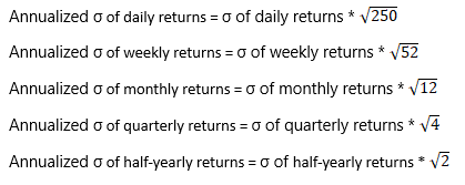
Keep in mind that in the above example, because we have used the daily returns data, we have multiplied the standard deviation by the square root of the number of trading days in a year. Had we instead used the weekly returns data, we would have multiplied the standard deviation by the square root of the number of weeks in a year. Similarly, had we instead used the monthly returns data, we would have multiplied the standard deviation by the square root of the number of months in a year. And so on. Let us summarize this as follows. (Kindly note that for daily period, the number of trading days could be something other than 250 also, depending up on holidays and weekends):
While the above calculation of standard deviation may look complex and time consuming, the good news is that you do not need to calculate standard deviation manually. You can just feed in the historical prices of the financial instrument of your choice in Microsoft Excel and the software will do all the work for you. Below mentioned are the steps for calculating standard deviation in Excel.
-
Download the historical price data of your choice in Excel format and open that Excel sheet. Some of the sites that I would recommend are www.nseindia.com, www.bseindia.com, in.finance.yahoo.com, and fred.stlouisfed.org
-
Assuming you have downloaded the daily data, I would suggest you sort them chronologically. Then, calculate the daily percent change of price using the formula mentioned below. The value that you get is the daily percent change. Do this for each of the day, as was shown in the table earlier.

-
Then click the insert function
 Once the insert function dialog box opens, type ‘std’ in the ‘search for a function’ box and press enter. This should show a list of functions that have the wording ‘std’ in them. Select the ‘STDEV’ function and press ok.
 -
Once the ‘function arguments’ dialog box opens, click on the number1 box. Then, go back to the excel sheet and select all the daily percent change data whose standard deviation you want to calculate.
-
Then, within the ‘function argument’ dialog box, press ok. The result (i.e. standard deviation) would be displayed.
Now that we understand how volatility (standard deviation) is calculated, let us proceed further and start discussing about how they are used in options parlance. In the world of options, the two most referred to volatilities are: historical volatility and implied volatility. In the next two sections, we will talk about each of these volatility types.
Historical Volatility
The calculations that we did in the previous section are nothing but those of historical volatility. Also known as statistical volatility, historical volatility measures the dispersion around the mean for daily returns on an annualized, percentage basis. It measures how volatile the movements in prices have been over the specified period. As stated earlier, the larger the movements, the higher is the historical volatility, and vice versa. Because historical volatility is expressed on an annualized, percentage basis, it can be used to compare the volatility between two or more securities. For instance, if the historical volatility of stock A is 12% while that of stock B is 18% over the same period, it tells that stock B has been more volatile than stock A.
Historical volatility is a very commonly used measure of risk. It tells how far from the mean the returns have fluctuated over time. This helps a trader in deciding the type of strategies that he could deploy as well as aid in setting up appropriate stop losses. For instance, when the volatility is low, a trader would know that he would be good with setting up a relatively small stop loss on the trade. However, when volatility is high, the trader would know the need to keep a larger stop loss to avoid being whipsawed due to the high levels of volatility. Keep in mind that there is a trade-off between profits and losses though. High volatility means high profit potential, but this comes at the cost of assuming the possibility of a higher loss too. Similarly, low volatility means the potential for low profits, but with the likelihood of lower losses as well.
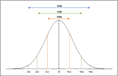
In the previous section, we saw that based on the daily returns data over a period of 30-trading days, the annualized standard deviation of Nifty was 9.51%. The question that one might ask is what exactly does this percent mean? What this means is that a one-standard deviation move in Nifty would take the index either 9.51% below or above the mean. Similarly, a two- standard deviation move in Nifty would take the index either 19.02% below or above the mean, and so forth. Statistically speaking, 68.2% of the data lies within one-standard deviation from the mean (34.1% on either side), 95.4% of the data lies within two-standard deviations from the mean (47.7% on either side), and 99.7% of data lies within three-standard deviations from the mean (49.8% on either side). The normally distributed chart below illustrates this:
So, for the example above, based on the recent 30-session price and return data, there is a ~68% probability of Nifty being within a range of ±9.51% (±1σ) from the mean return over a one-year period, ~95% probability of Nifty being within a range of ±19.02% (±2σ) from the mean return, and a ~99% probability of Nifty being within a range of ±28.53% (±3σ) from the mean return. Looking at it the other way, there is a ~32% chance of Nifty moving beyond ±9.51% (±1σ) range from the mean return over a one-year period, ~5% chance of Nifty moving beyond ±19.02% (±2σ) from the mean return, and a less than 1% probability of Nifty moving beyond ±28.53% (±3σ) from the mean return.
Implied Volatility
Historical volatility is a very useful measure of risk. However, it is not used for the pricing of options, given that it is backward-looking and not forward-looking. Instead, the volatility that is used for the pricing of options is known as Implied Volatility (or IV). Implied volatility is used to measure future volatility.It is based on what market participants imply the volatility of the underlying will be over the remaining life of an option contract.So, while historical volatility calculates the past changes in the underlying, implied volatility measures the possibility of future changes in the price of the underlying. It is the market participant’s forecast of how a security’s price could change over time based on a certain set of parameters. Just like historical volatility, implied volatility is expressed as a percentage on an annualized basis.
Implied Volatility is very crucial to options trading because it enables one to understand what the market is perceivingabout the underlying’s future move, regardless of the direction of that move. For instance, if the implied volatility for an underlying is rising and is higher than historic levels, it informs an option trader that market participants are expecting volatility to pick up ahead, which could be due to numerous factors such as potential news that is/are expected to come out, events that are lined up in future, some major announcements that could be made etc. Whatever the reasons, rising implied volatility means that market participants anticipate the trading range to expand, which in turn will cause the option price to move, irrespective of whether the underlying price has moved or not. Keep in mind that the time value component of an option price could change even if there is not much of a movement in the underlying price, for factors such as changing volatility, time decay etc.
Rising implied volatility usually causes the price of an option to increase in value, while falling implied volatility usually causes the price of an option to decrease in value. Hence, rising volatility tends to benefit an option holder, while falling volatility tends to benefit an option writer. As stated, implied volatility is expressed as a percentage on an annualized basis. As an example, if the implied volatility is 15% and if the current underlying price is ₹100, a one standard deviation move would mean the underlying would be in a range of ₹85 to ₹115 over the next one year. If the IV increases, so would the trading range on an annualized basis, and vice versa. Given that most of the option trading on Indian exchanges are usually short-term, one can convert the annualized implied volatility into the desired time frame, depending upon the days left to expiration of the option contract. The formula that one can use to calculate the custom-period volatility is:

For instance, if the implied volatility is 15% and the time left to expiration is 1-month, the 1-month implied volatility can be calculated as:

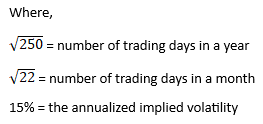
As can be seen, the 1-month IV is 4.45%, meaning that there is a 68% probability of the underlying price being within a range of ±4.45% from the current price over the next one month.
Concluding this Topic
The objective of this chapter was to just introduce the concept of Volatility. In this chapter, we saw what volatility is, we saw that standard deviation is the most widely used measure of volatility, we saw how to calculate and interpret standard deviation, we saw how to annualize standard deviation, we saw how to calculate standard deviation in Microsoft Excel, and finally we saw what historical and implied volatility are. In the next chapter, we shall turn focus back towards Options Greek and talk about Vega.
Next Chapter
Comments & Discussions in
FYERS Community

